Support Vector Machine is the so-called SVM. It refers to a series of machine learning algorithms. According to the different problems solved, it is divided into SVC (classification) and SVR (regression).
SVC, Support Vector Classification, is essentially a support vector machinesupport vector, but it is only used for classificationclassificationTask
SVR, Support Vector Regression, its essence is also a support vector machinesupport vector , only for regressionRegressiontask
This column is mainly a summary of classification algorithms. Mainly introduce SVC
C-Support Vector Classification (C-Support Vector Classifier) is implemented based on libsvm. The fitting time has at least a quadratic relationship with the number of samples, and may not be feasible beyond tens of thousands of samples. For large data sets, consider using LinearSVC or SGDClassifier, possibly after using the Nystroem transformer or other kernel approximation methods.
1. Algorithm idea
Take the two-classification task as an example. There are two different types of sample data. A new sample is received and classified. Here are some core concepts, described in my own vernacular.
Find a line that can divide the sample data of these two categories. This line is called the decision boundary
Take the decision boundary as the center and translate to both sides. Until the sample point is touched, the interval between the two lines is called margin (interval); the sample point touched is called the support vector
and finally becomes< a i=3>Find the largest marginProblem
Decision boundary: Find a line (two-dimensional) that can divide the two categories of data, or a hyperplane (three-dimensional), etc.
Interval: Center the decision boundary Translate on both sides until it hits the nearest sample point. The distance between these two lines is margin (interval)
Support vector: Translate to both sides with the decision boundary as the center. These two lines The sample points encountered are called support vectors
Hard interval: rigid interval, the interval obtained by strictly following the algorithm solution idea
Soft interval: flexible interval, if there is an outlier or noise point, it can be restricted based on regularization to get a consistent
The blue noise here should belong to the pentagon category, but it is a five-pointed star category in the data set sample. This sample is a noise point, which will affect the normal classification and needs to be eliminated. At this time, a soft interval is introduced to reduce the The impact of noise.

2. Official website API
class sklearn.svm.SVC(*, C=1.0, kernel='rbf', degree=3, gamma='scale', coef0=0.0, shrinking=True, probability=False, tol=0.001, cache_size=200, class_weight=None, verbose=False, max_iter=-1, decision_function_shape='ovr', break_ties=False, random_state=None)
There are quite a lot of parameters here. For specific parameter usage, you can learn based on the demo provided on the official website and try it more; here are some commonly used parameters for explanation.
Guide package:from sklearn.svm import SVC
①Regularization parameter C
The strength of the regularization is inversely proportional to the regularization parameter C. The penalty is the square of the L2 regularization. C is a floating point number type.
The specific official website details are as follows:

Usage
SVC(C=2.0)
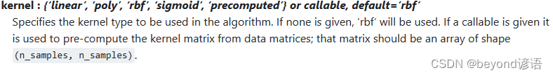
②Kernel function kernel
'linear': linear kernel function, fast; can only process data set sampleslinear separable, cannot handle linear inseparability.
'poly': Polynomial kernel function, which can increase the dimension of data set samples and map from low-dimensional space to high-dimensional space. Dimensional space; many parameters, large amount of calculation
'rbf': Gaussian kernel function, the same as polynomial kernel function , can increase the dimension of the sample; compared with the polynomial kernel function, it has fewer parameters; the default value
'sigmoid
< a i=13>': sigmoid kernel function; when using the sigmoid kernel function, SVM can implement a multi-layer neural network 'precomputed ': Kernel matrix; use the kernel function matrix (n*n) given by the user
You can also customize your own kernel function and then call it
The specific official website details are as follows:
Usage
SVC(kernel='sigmoid')
③The degree of the polynomial kernel function
The order of the polynomial kernel function; this parameter is only useful for the polynomial kernel function (poly); if it is other kernel functions, the system will This parameter is automatically ignored
The specific official website details are as follows:

Usage
SVC(kernel='ploy',degree=2)
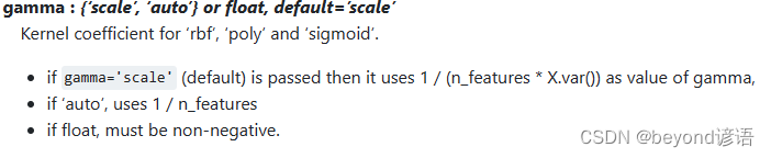
④Kernel coefficient gamma
rbf, poly and sigmoidThe kernel coefficient of the kernel function. This parameter is only for these three kernel functions. Please note that
' or other floating point numbers can be used': For the specific calculation formula, please see the official website details below auto '': Default value, for the specific calculation formula, please see the official website details belowscale
The specific official website details are as follows:
Usage
SVC(gamma='auto')
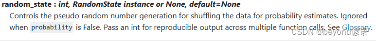
⑤Random seed random_state
If you need to control variables for comparison, it is best to set the random seed here to the same integer.
The specific official website details are as follows:
Usage
SVC(random_state=42)
⑥Finally build the model
SVC(C=3.0,kernel=‘sigmoid’,gamma=‘auto’,random_state=42)
3. Code implementation
①Guide package
Here you need to evaluate, train, save and load the model. The following are some necessary packages. If an error is reported during the import process, just install it with pip.
import numpy as np
import pandas as pd
import matplotlib.pyplot as plt
import joblib
%matplotlib inline
from sklearn.model_selection import train_test_split
from sklearn.svm import SVC
from sklearn.metrics import confusion_matrix, classification_report, accuracy_score
②Load the data set
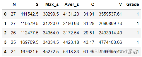
The data set can be simply created by itself in csv format. What I use here is 6 independent variables X and 1 dependent variable Y.
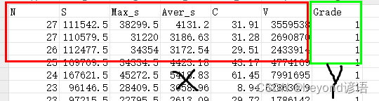
fiber = pd.read_csv("./fiber.csv")
fiber.head(5) #展示下头5条数据信息
③Divide the data set
The first six columns are the independent variable X, and the last column is the dependent variable Y
Official API of commonly used split data set functions:train_test_split
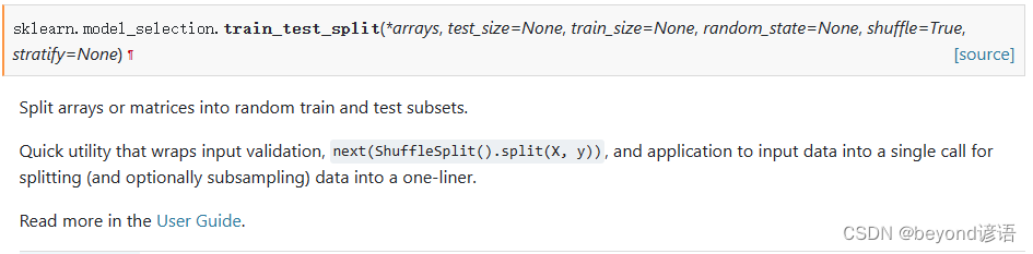
test_size: Proportion of test set data
train_size: Proportion of training set data
random_state: Random seed
shuffle: Whether to disrupt the data
Because my data set here has a total of 48, training set 0.75, test set 0.25, that is, 36 training sets and 12 test sets
X = fiber.drop(['Grade'], axis=1)
Y = fiber['Grade']

X_train, X_test, y_train, y_test = train_test_split(X,Y,train_size=0.75,test_size=0.25,random_state=42,shuffle=True)

print(X_train.shape) #(36,6)
print(y_train.shape) #(36,)
print(X_test.shape) #(12,6)
print(y_test.shape) #(12,)
④Build SVC model
You can try setting and adjusting the parameters yourself.
svc = SVC(C=3.0,kernel='sigmoid',gamma='auto',random_state=42)
⑤Model training
It’s that simple, a fit function can implement model training
svc.fit(X_train,y_train)
⑥Model evaluation
Throw the test set in and get the predicted test results
y_pred = svc.predict(X_test)
See if the predicted results are consistent with the actual test set results. If consistent, it is 1, otherwise it is 0. The average is the accuracy.
accuracy = np.mean(y_pred==y_test)
print(accuracy)
can also be evaluated by score. The calculation results and ideas are the same. They all look at the probability of the model guessing correctly in all data sets. However, the score function has been encapsulated. Of course, the incoming The parameters are also different, you need to import accuracy_score, from sklearn.metrics import accuracy_score
score = svc.score(X_test,y_test)#得分
print(score)
⑦Model testing
Get a piece of data and use the trained model to evaluate
Here are six independent variables. I randomly throw them alltest = np.array([[16,18312.5,6614.5,2842.31,25.23,1147430.19]])
into the model. Get the prediction result, prediction = svc.predict(test)
See what the prediction result is and whether it is the same as the correct result, print(prediction)
test = np.array([[16,18312.5,6614.5,2842.31,25.23,1147430.19]])
prediction = svc.predict(test)
print(prediction) #[2]
⑧Save the model
svc is the model name, which needs to be consistent
The following parameter is the path to save the model
joblib.dump(svc, './svc.model')#保存模型
⑨Load and use the model
svc_yy = joblib.load('./svc.model')

test = np.array([[11,99498,5369,9045.27,28.47,3827588.56]])#随便找的一条数据
prediction = svc_yy.predict(test)#带入数据,预测一下
print(prediction) #[4]
Complete code
Model training and evaluation does not include ⑧⑨.
from sklearn.svm import SVC
import pandas as pd
import numpy as np
from sklearn.model_selection import train_test_split

fiber = pd.read_csv("./fiber.csv")
# 划分自变量和因变量
X = fiber.drop(['Grade'], axis=1)
Y = fiber['Grade']
#划分数据集
X_train, X_test, y_train, y_test = train_test_split(X, Y, random_state=0)

svc = SVC(C=3.0,kernel='sigmoid',gamma='auto',random_state=42)
svc.fit(X_train,y_train)#模型拟合
y_pred = svc.predict(X_test)#模型预测结果
accuracy = np.mean(y_pred==y_test)#准确度
score = svc.score(X_test,y_test)#得分
print(accuracy)
print(score)

test = np.array([[23,97215.5,22795.5,2613.09,29.72,1786141.62]])#随便找的一条数据
prediction = svc.predict(test)#带入数据,预测一下
print(prediction)