Introduction to knowledge integration
Knowledge fusion, that is, merging two knowledge graphs (ontologies), the basic problem is to study how to fuse description information about the same entity or concept from multiple sources. What needs to be confirmed are: equivalent instances, equivalent classes/subclasses, and equivalent attributes/subattributes.
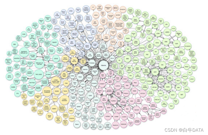
An example is shown in the figure above. The circles of different colors in the figure represent different knowledge graph sources. Rome in dbpedia.org and roma in geoname.org are the same entity and are linked through two sameAs. Entity alignment between different knowledge graphs is the main work of KG fusion.
In addition to entity alignment, there is also work on conceptual level knowledge fusion and cross-language knowledge fusion.
It is worth mentioning here that in different literatures, knowledge fusion has different names, such as ontology alignment, ontology matching, Record Linkage, Entity Resolution, entity alignment, etc., but their essential work is the same.
The main technical challenges of knowledge fusion are two points:
1. Data quality challenges: such as ambiguous naming, data entry errors, data loss, inconsistent data formats, abbreviations, etc.
2. Challenges of data scale: large amount of data (parallel computing), diversity of data types, no longer just name matching, multiple relationships, more links, etc.
Basic technical process
Knowledge fusion is generally divided into two steps. The basic processes of ontology alignment and entity matching are similar, as follows:
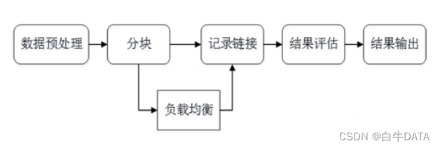
1. Data preprocessing
In the data preprocessing stage, the quality of the original data will directly affect the final link result. Different data sets often describe the same entity in different ways. Normalizing these data is an important step to improve the accuracy of subsequent links. .
Commonly used data preprocessing include:
1. Grammar regularization
2. Grammar matching: such as the representation method of contact number
3. Comprehensive attributes: such as the expression of home address
4. Data normalization
5. Remove spaces, "", "", - and other symbols
6. Topological errors of the input error class
7. Replace nicknames, abbreviations, etc. with formal names
2. Record the connection
Assume that the records x and y of two entities have the values of x and y on the i-th attribute. Then the record connection is performed in the following two steps:
Attribute similarity: Combining the similarity of individual attributes to obtain the attribute similarity vector:
Entity similarity: Obtain the similarity of an entity based on the attribute similarity vector
Calculation of attribute similarity
There are many methods for calculating attribute similarity. Commonly used ones include edit distance, set similarity calculation, vector-based similarity calculation, etc.
1. Edit distance: Levenstein, Wagner and Fisher, Edit Distance with Afine Gaps
2. Set similarity calculation: Jaccard coefficient, Dice
3. Vector-based similarity calculation: Cosine similarity, TFIDF similarity
Edit distance calculates attribute similarity
Levenshtein distance, that is, the minimum edit distance, aims to convert one string into another with the least editing operations. For example, calculate the edit distance between Lvensshtain and Levenshtein: Lvensshtain is converted to Levenshtein, a total of 3 operations, and the edit distance is also That’s 3. LevensteinDistance is a typical dynamic programming problem and can be calculated by the dynamic programming algorithm, where +1 represents the cost of insertion, deletion and replacement operations.
Wagner and Fisher Distance is an extension of Levenshtein distance, which assigns different weights to the cost of editing operations in this model, where del, ins, and sub are the costs of deletion, insertion, and replacement respectively.
Edit Distance with affine gaps is based on the above two algorithms and introduces the concept of gap. The above insertion, deletion and replacement operations are replaced by gap opening and gap extension, where s is the cost of open extension and e is the cost of extend gap. Cost, l is the length of the gap. For example, to calculate the distance between Lvensshtain and Levenshtein, first align the two words head to tail, and regard the corresponding missing parts as gaps. Compared with the words below, the first e and the third e from the bottom are missing. These are two gap. The word below has one less s and a than the word above, which is another two gaps. Together, there are 4 gaps, each with a length of 1.
Set similarity calculation attribute similarity
The Dice coefficient is used to measure the similarity of two sets. Because strings can be understood as a set, the Dice distance is also used to measure the similarity of strings. The Dice coefficient takes Lvensshtain and Levenshtein as examples. The similarity between the two The degree is 2 * 9 / (11+11)= 0.82.
The Jaccard coefficient is suitable for processing the similarity of short texts and is similar to the definition of the Dice coefficient. There are two methods to convert text into sets. In addition to using symbols to divide words, you can also consider using n-grams to divide words, n-grams to divide sentences, etc. to build sets and calculate similarities.
TF-IDF's vector-based similarity is mainly used to evaluate the importance of a certain word or word to a document. For example, there are 50,000 articles in a certain corpus, and 20,000 articles contain "health". There is one article with a total of 1,000 words, and "health" appears 30 times, then sim TF-IDF =30/1000 * log( 50000/(20000+1)) = 0.012.
Calculation of entity similarity
Calculating entity similarity can start from three major aspects, namely aggregation, clustering and representation learning.
1. Aggregation: Weighted average method, that is, weighted summation of each component of the similarity score vector to obtain the final entity similarity: Manually formulating rules is to set a threshold for each component of the similarity vector. If the threshold is exceeded, Connect two entities:
For machine learning methods such as classifiers, the biggest problem is how to generate a training set. For this, unsupervised/semi-supervised training can be used, such as EM, generative models, etc. Or active learning solutions such as crowdsourcing.
2. Clustering: Clustering can be divided into hierarchical clustering, correlation clustering, Canopy + K-means, etc.
Hierarchical Clustering divides data at different levels by calculating the similarity between different categories of data points, and finally forms a tree-like clustering structure.
The underlying original data can be calculated through the similarity function. There are three algorithms for similarity between classes:
SL (Single Linkage) algorithm: The SL algorithm, also known as the nearest-neighbor algorithm, uses the similarity between the two closest data points among the two classes of data points as the distance between the two classes.
CL (Complete Linkage) algorithm: Different from SL, the similarity of the two furthest points in the two classes is taken as the similarity of the two classes.
AL (Average Linkage) algorithm: uses the average similarity between all points in two classes as the inter-class similarity.
Correlation clustering indicates that x and y are assigned to the same class, represents the probability that x and y are in the same class (similarity between x and y), and are respectively the cost and retention of cutting off the edge between x and y Side price. The goal of correlation clustering is to find a clustering solution with the minimum cost. It is an NP-Hard problem and can be approximately solved by the greedy algorithm.
Canopy + K-means is different from K-means. The biggest feature of Canopy clustering is that it does not need to specify the k value (that is, the number of clustering) in advance. Therefore, it has great practical application value. Canopy and K-means are often used together. .
3. Representation learning: Map the entities and relationships in the knowledge graph to low-dimensional space vectors, and directly use mathematical expressions to calculate the similarity between each entity. This type of method does not rely on any text information and obtains the deep features of the data.
There are many ways to map two knowledge graphs to the same space. Their bridge is pre-connected entity pairs (training data). For details, please see the detailed paper.
How to perform entity linking after completing the mapping? After KG vector training reaches a stable state, for each entity in KG1 that has not found a link, find the entity vector closest to it in KG2 for linking. The distance calculation method can use the distance calculation between any vectors, such as Euclidean distance or Cosine distance.
3. Chunking
Blocking is to select potentially matching record pairs as candidates from all entity pairs in a given knowledge base, and reduce the size of the candidates as much as possible. The reason for this is simply because there is too much data. . . It is impossible for us to connect them one by one.
Commonly used blocking methods include blocking based on Hash function, adjacent blocking, etc.
First, we introduce chunking based on Hash function. For record x, there is , then x is mapped to the block bound to the keyword. Common Hash functions are:
1. The first n characters of the string
2.n-grams
3. Combine multiple simple hash functions, etc.
4. Neighboring blocking algorithms include Canopy clustering, sorted neighbor algorithm, Red-Blue SetCover, etc.
4. Load balancing
Load Balance (Load Balance) ensures that the number of entities in all blocks is equal, thereby ensuring the performance improvement of block partitioning. The simplest method is multiple Map-Reduce operations.
Tool introduction
1. Ontology Alignment - Falcon-AO
Falcon-AO is an automatic ontology matching system that has become a practical and popular choice for matching Web ontologies expressed in RDF(S) and OWL. The programming language is Java.
The matching algorithm library includes four algorithms: V-Doc, I-sub, GMO, and PBM. Among them, V-Doc is linguistic matching based on virtual documents. It is a collection of entities and surrounding entities, nouns, texts and other information to form a virtual document. In this way we can operate with algorithms such as TD-IDF. I-Sub is a string matching based on edit distance, which we have introduced in detail earlier. It can be seen that both I-Sub and V-Doc are based on string or text level processing. A further step is GMO, which matches the graph structure of RDF ontology. PBM is based on the idea of divide and conquer.
2. Limes entity matching
Limes is an entity matching discovery framework based on metric space, suitable for large-scale data linking, and the programming language is Java.