The Huawei Cup Research Competition CDEF question idea model and code have been updated throughout the entire process. Please check the business card at the end of the article to obtain it.
Analysis of Huawei Cup Question C Ideas
Question 1: At each review stage, works are usually randomly distributed, and each work requires independent review by multiple judges. In order to increase the comparability of the scores given by different review experts, there should be some overlap between the collections of works reviewed by different experts. But if some intersections are large, there must be some intersections that are small, and comparability becomes weaker. Please establish a mathematical model to determine the optimal "cross-distribution" plan based on the situation of 3,000 participating teams and 125 review experts, and each work is reviewed by 5 experts, and discuss the relevant indicators (your own definition) and implementation details of the plan .
Problem one mainly involves establishing an optimal "cross-distribution" plan for 3,000 participating teams and 125 review experts. The key here is to ensure that each work is reviewed by 5 experts, and that there is a certain overlap between the collections of works reviewed by different experts. This problem can be regarded as a combinatorial optimization problem. We can use a graph theory model to model it as a vertex coloring problem of the graph and solve it to obtain the optimal "cross distribution" solution .
Our variable is defined as a binary variable xij , which is 1 when the i-th expert reviews the j-th work, and 0 otherwise.
Our objective function is to maximize the size of the intersection of works among all experts, that is, to maximize
![]()
We give the constraint that each work is reviewed by exactly 5 experts; the number of works reviewed by each expert should be evenly distributed to prevent a certain expert from being overly heavy or too light.
This is an NP-hard problem, and we can apply heuristic algorithms such as genetic algorithms and simulated annealing algorithms to solve it. These algorithms are suitable for searching the solution space of large-scale combinatorial optimization problems and can find satisfactory solutions within a reasonable time.
Question 2 uses a ranking method based on standard scores (Appendix 1) in the review, which assumes that the academic level distribution of the collections of works reviewed by different review experts is the same. However, in the review of large-scale innovation competitions, usually only a small part of the works reviewed by any two experts are in common, and the vast majority of the works are different (see question 1), and each expert only sees a small collection of works. Therefore, the assumptions of the standard sub-evaluation scheme may not be valid, and new evaluation schemes need to be explored. Please select two or more existing or self-designed review plans and question attachment data, analyze the distribution characteristics of the original scores of each expert and each work, and the scores after adjustment (such as standard scores), and sort according to different plans , and try to compare the pros and cons of these options. Then, a new standard score (formula) calculation model is designed for the review of large-scale innovation competitions. In addition, it is generally believed that award-winning papers that have been unanimously agreed upon by multiple experts have the greatest credibility. For the data 1 provided in Appendix 2, the ranking of the first-prize works selected in the second review stage was reached through expert consultation. Please use This batch of data will improve your standard score calculation model.
Question two involves comparing and analyzing different review schemes and designing a new standard score calculation model based on the given data. We can analyze several existing review schemes and compare the advantages and disadvantages of these schemes using methods such as descriptive statistics and hypothesis testing. , such as mean, median, standard deviation, etc., to analyze the distribution characteristics of the original scores and adjusted scores of each expert and each work. We make some visual displays of the score distribution under different plans to more intuitively understand the differences between different plans.
In order to determine whether the differences between different scenarios are significant, we can use hypothesis testing methods. Use ANOVA (Analysis of Variance) to compare whether there are significant differences in the mean scores of multiple programs. Use the chi-square test or Fisher's exact test to compare differences in the distribution of grades under different programs.
Then based on these analysis results, we design a new standard score calculation model. For this problem , we can consider using regression analysis. In addition to using regression analysis, we can also build an optimization model to solve the optimal standard score calculation method. The objective function of this model can be to minimize the variance of the standard scores of all works to reduce the differences between different solutions. Constraints can include maintaining fairness in scoring and maintaining a certain degree of diversity.
Question 3: The characteristic of the "Innovation" competition is "innovation", that is, there is no standard answer. Since the problems in this type of competition are difficult, they generally require innovation to be partially solved during the competition. It is difficult to agree on the extent of the innovation of the work and the prospects for subsequent research. Even if experts communicate face-to-face, they may not be able to unify due to their own opinions. In addition, the graduate students' papers are not well expressed and the review experts have different perspectives. The scores given by several experts on the same work will be quite different (extremely poor). Large ranges are a characteristic of large-scale innovation competitions. Works with relatively large ranges are generally in high or low categories. Low-segmented items belong to the elimination range. The reason for the large difference in low-segmented items is that some experts have given very low scores to works that violate regulations or have major mistakes, or the review experts all agree that the quality of the work is not high, but one of them ( Some) experts even disagree with the work. Therefore, although the range here is large, it falls within the category of non-award-winning, and generally does not need to be adjusted. High-segmented works must also participate in the more authoritative second-stage review (the same row in the attached data table represents the results of the same work in the two stages. Works without second-stage review scores only participated in the first-stage review. ). In the second stage of the review, there are still some works with large differences. Because it is the final review, the errors may affect the award level. Therefore, some works with large differences need to be reconsidered and adjusted (the data in the attachment are recorded, and the review score is the expert's). The final standard score is used to replace the original standard score). In the second stage (note that the number of review experts for each work is different in the two stages), the rules for experts to adjust the "large range" can be used as a reference for establishing a range model.
Based on the simulation data 2.1 and 2.2 given in the question, please discuss the overall changes in the two-stage scores and the overall changes in the two-stage extremes, and analyze the advantages and disadvantages of the two-stage evaluation plan compared to the non-stage evaluation plan. Notice that there is a certain relationship between the two characteristics of large range and strong innovation. In order to discover innovative papers, please establish a "range" model (including analysis, classification, adjustment, etc.), and try to give the given data The first review stage is a programmed (without manual intervention) method of handling the "large difference" of works that are not high and not low.
For question three , we will focus on the comparison between the two-stage review plan and the non-stage review plan, as well as the establishment of the "extremely poor" model. It is necessary to analyze the performance changes and range changes in the two stages, and explore how to deal with the "large range".
To compare the two-stage evaluation plan and the non-stage evaluation plan , you can use analysis of variance (ANOVA) to compare the difference in scores between the two-stage evaluation plan and the non-stage evaluation plan, and test whether there is a significant difference in the mean scores under different plans, and these Whether the differences can be attributed to the review scheme used
Then calculate their mean, standard deviation, interquartile range and other descriptive statistics, so that you can understand the difference in score distribution between the two programs in more detail. And these differences can be demonstrated through visualization tools such as box plots and histograms .
To build a range model, you can use either classification or clustering. First, use the classification model. Let's predict the range size of the work. By inputting various characteristics of the work (such as preliminary scores from experts, type of work, etc.), the classification model can predict whether the extreme difference of the work will exceed a certain threshold. As for algorithms, you can use decision trees, random forests, support vector machines, etc. Finally, cross-validation is used to select the best model and parameters.
With cluster analysis, we can group works with similar extremely poor characteristics into the same category. It allows us to understand which works are more likely to produce large extreme differences. The clustering algorithm can use K-means clustering or hierarchical clustering.
Analysis of Huawei Cup question D ideas
Question 1: Analysis of the current situation of regional carbon emissions, economy, population, and energy consumption
(1) Establish indicators and indicator systems
Requirement 1: The indicator can describe the economy, population, energy consumption and carbon emissions of a certain region;
Requirement 2: The indicator can describe the carbon emission status of each department (energy supply department, industrial consumption department, construction consumption department, transportation consumption department, residential consumption department, agriculture and forestry consumption department);
Requirement 3: The indicator system can describe the interrelationship between the main indicators;
Requirement 4. Changes in some indicators (year-on-year or month-on-month) can become the basis for carbon emission predictions.
We can consider the following for indicator selection :
Economic indicators: GDP growth rate is selected as the main indicator to measure regional economic conditions. It can comprehensively reflect the level of economic development and the activity of economic activities in a region.
Population indicators: Total population and population growth rate are important indicators for evaluating population status. They can reflect the size and growth rate of regional population and have a direct impact on energy consumption and carbon emissions.
Energy consumption indicators: Total energy consumption and energy consumption structure (the ratio of fossil energy to non-fossil energy) are key indicators to measure energy consumption. They directly affect the size and structure of carbon emissions.
Carbon emission indicators: Total carbon emissions, carbon emissions per unit of GDP and carbon emissions of each department are the main indicators to evaluate the carbon emission status. They can comprehensively describe the carbon emission level and structure of a region.
Sector division: The entire region is divided into the energy supply sector, industrial consumption sector, construction consumption sector, transportation consumption sector, residential consumption and agriculture and forestry consumption sectors, and the energy consumption and carbon emissions of each sector are independently analyzed.
After selecting indicators, it is necessary to establish a relationship model between these indicators. A multiple linear regression model can be used here, using carbon emissions as the dependent variable and the remaining indicators as independent variables to establish the mathematical relationship between them. For example, you can explore the impact of GDP growth rate, population growth rate and energy consumption structure on carbon emissions, and analyze the sensitivity and elasticity between them. For selected indicators, their year-on-year and month-on-month changes are calculated, and these changes can serve as the basis for carbon emission forecasts. If energy consumption increases significantly in a given year, carbon emissions are likely to increase that year as well. By analyzing these changes, we can better understand the impact of each indicator on carbon emissions.
(2) Analyze the current status of regional carbon emissions, economy, population, and energy consumption
Requirement 1: Using 2010 as the base period, analyze the 12th Five-Year Plan (2011-2015) and the 13th Five-Year Plan for a certain region
Carbon emission status (such as total amount, change trend, etc.) during the period (2016-2020);
Requirement 2: Analyze the factors that affect carbon emissions in the region and their contributions;
Requirement 3: Analyze and determine the main challenges that the region needs to face to achieve carbon peaking and carbon neutrality, and provide a basis for differentiated path selection in the region’s dual-carbon (carbon peaking and carbon neutrality) path planning.
Using existing historical data, we can analyze the changing trends and conditions of regional carbon emissions, economic growth, population growth and energy consumption from 2010 to 2020. Through methods such as graphing and calculating growth rates, we can clearly see the development trajectory of these indicators, thereby gaining a preliminary understanding of the current carbon emissions in this region. Then we analyze the impact of changes in various indicators on carbon emissions and find out the main driving factors for the growth of carbon emissions.
For models, statistical methods such as correlation analysis and regression analysis can be used to quantify the contribution of each factor to carbon emissions. We can analyze the contribution of economic growth to carbon emissions and determine whether economic development is the main reason for the growth of carbon emissions.
Of course, there are other external factors, such as government policies, technological progress, etc., which will also affect changes in carbon emissions. Based on the analysis of the current situation and understanding of the influencing factors, we can predict the main challenges in achieving carbon peak and carbon neutrality in this region. Including difficulties in energy structure adjustment, restrictions on the development of non-fossil energy, conflicts between economic development and carbon emission reduction , etc.
(3) Regional carbon emissions, economic, population, energy consumption indicators and their correlation models
Requirement 1: Analyze changes in relevant indicators (month-on-month and year-on-year);
Requirement 2: Establish a relationship model between various indicators;
Requirement 3: Based on changes in relevant indicators, combined with multiple effects such as dual-carbon policy and technological progress, determine the values of carbon emission prediction model parameters (such as energy utilization efficiency improvement and the proportion of non-fossil energy consumption, etc.).
After analyzing the current status and influencing factors of each indicator, we need to establish a correlation model between each indicator. Here, methods such as multiple linear regression and principal component analysis can be used to fit the mathematical relationship between various indicators based on historical data.
We use carbon emissions as the dependent variable, GDP, population, energy consumption, etc. as independent variables, and establish linear and nonlinear models between them through regression analysis. It can help us understand the interaction between various indicators. After establishing the correlation model, we need to determine the parameters in the model. These parameters include energy utilization efficiency, proportion of non-fossil energy consumption, etc. They are the core components of the model and directly affect the prediction effect of the model.
Question 2: Forecasting model of regional carbon emissions, economy, population, and energy consumption
(1) Energy consumption forecast model based on demographic and economic changes
Requirement 1: Using 2020 as the base period and combining the two time nodes of Chinese-style modernization (2035 and 2050), predict the population, Changes in the economy (GDP) and energy consumption.
Requirement 2: Energy consumption is linked to population projections.
Requirement 3: Energy consumption is linked to economic (GDP) forecasts;
The Huang Futao model can be chosen to predict future population size. The model takes into account the effects of factors such as birth rate and death rate.
Pt+1 = Pt + Bt - Dt + It - Et
We can also use population prediction models such as logarithmic linear models or logistic models, combined with regional historical population data, to predict future population change trends. Of course, we need to consider factors that may have an impact, such as fertility rate, mortality rate, and migration rate . During the prediction process, model parameters must be continuously adjusted to ensure the accuracy of the prediction results.
Economic (GDP) forecasting can use time series analysis, multiple regression analysis and other methods, combined with national macroeconomic policies, global economic situation, etc., to predict the future economic development trend of the region.
G(t) = G0 / [1 + ae^(-bt)]
Energy consumption forecasting needs to be combined with predicted population and economic data, and methods such as cointegration analysis and causal models should be used to predict future energy consumption.
E(t) = c1P(t) + c2G(t) - c3*E'(t)
(2) Regional carbon emissions prediction model
Requirement 1: Carbon emissions are related to population, GDP and energy consumption forecasts;
Requirement 2: Carbon emissions and various energy consumption sectors (industrial consumption sector, construction consumption sector, transportation
consumption sector, residential consumption, agriculture and forestry consumption sector) and the energy supply sector (such as reflecting the impact of energy efficiency improvements on the distribution of total energy consumption in the above energy consumption sectors);
Requirement 3: Carbon emissions and energy consumption types (primary energy) in each energy consumption sector (same as above)
Fossil energy consumption is related to non-fossil energy consumption and secondary energy (electricity or heat) consumption) and the types of energy consumption in the energy supply sector (fossil energy power generation and non-fossil energy power generation) (such as reflecting the impact of the increase in the proportion of non-fossil energy consumption on each The impact of sectoral energy consumption types or carbon emission factors).
We need to first establish a relationship model between carbon emissions and population, GDP and energy consumption. Here you can consider using multiple regression analysis, using carbon emissions as the dependent variable and population, GDP and energy consumption as independent variables to fit the relationship between them. We can then quantify the impact of population, economy and energy consumption on carbon emissions to predict future changes in carbon emissions.
It is also necessary to establish carbon emission prediction models for each energy consumption sector (such as industry, construction, transportation, etc.), taking into account the impact of energy consumption, energy consumption structure and other factors in each sector.
Analyze the impact of the increase in the proportion of non-fossil energy consumption on energy consumption types or carbon emission factors in various departments. This requires us to conduct in-depth research on the carbon emission characteristics of non-fossil energy and its application in different sectors. To evaluate the emission reduction effect of increasing the proportion of non-fossil energy consumption .
Finally, we also need to validate the model to test its predictive ability and accuracy. If the model prediction results are consistent with the actual data, the model is effective; if not, the model needs to be adjusted.
Analysis of ideas for question E
- Exploratory modeling of factors associated with hematoma expansion risk.
Please use "Table 1" (fields: serial number of the first imaging examination after admission, time interval from onset to first imaging examination) and "Table 2" (fields: serial numbers at each time point and corresponding HM_volume) to determine after the onset of patients sub001 to sub100 Whether a hematoma expansion event occurred within 48 hours.
Result filling specifications : 1 yes, 0 no, filling position: field C of "Table 4" (whether hematoma expansion occurs).
If a hematoma expansion event occurs, please also record the time when the hematoma expansion occurred.
Result filling specifications : For example, 10.33 hours, filling position: "Table 4" field D (hematoma expansion time).
Whether hematoma expansion occurs can be based on the changes in hematoma volume, which is specifically defined as: an absolute volume increase of ≥6 mL or a relative volume increase of ≥33% in subsequent examinations compared with the first examination.
Note: You can query the corresponding imaging examination time point through the serial number to "Appendix 1 - Search Form - Serial Number vs Time", and combine the time interval from onset to the first imaging and the subsequent imaging examination time interval to determine whether the current imaging examination is during the onset of illness 48 Within hours.
Extract the "serial number of the first imaging examination upon admission" and the "time interval from onset to first imaging examination" from "Table 1".
Extract the "serial number" and corresponding "HM_volume" at each time point from "Table 2". Use "Appendix 1 - Search Form - Serial Number vs Time" to query the image inspection time point corresponding to each serial number.
For each patient, identify all imaging studies within 48 hours of onset of illness. Compare the "HM_volume" of these imaging examinations with the "HM_volume" of the first imaging examination to determine whether the conditions for hematoma expansion are met (absolute volume increase ≥6 mL or relative volume increase ≥33%). If hematoma expansion occurs, the time of occurrence is recorded; otherwise, hematoma expansion is marked as not occurring.
Please use whether a hematoma expansion event occurs as the target variable, based on the personal history, disease history, onset-related (fields E to W) of the first 100 patients (sub001 to sub100) in "Table 1", and their imaging examination results in "Table 2" (Fields C to Probability.
Note: This question can only include the patient’s first imaging examination information.
Result filling specifications : record the predicted probability of event occurrence (value range 0-1, retain 4 digits after the decimal point); fill in location: "Table 4" field E (predicted probability of hematoma expansion).
We first perform feature selection and select the patient's personal history, disease history, and disease-related characteristics from "Table 1". Select the relevant characteristics of the first imaging examination from "Table 2" and "Table 3".
Then you can use machine learning methods for classification. There are many models available here, such as logistic regression, support vector machine, random forest, gradient boosting, etc. We use these models to do a cross-validation and parameter tuning to select Optimal model and parameters.
Use the data of the first 100 patients as the training set for model training. Use the cross-validation method to evaluate the performance of the model on the training set, and examine the accuracy, recall, F1 score, etc. of the model. Finally, predict the probability of hematoma expansion for all patients (sub001 to sub160).
- Model the occurrence and progression of perihematoma edema, and explore the relationship between therapeutic intervention and edema progression.
- Please construct an edema volume progression curve over time for all patients based on the edema volume (ED_volume) and repeated examination time points of the first 100 patients (sub001 to sub100) in "Table 2" (x-axis: time from onset to imaging examination, y-axis: Edema volume, y=f(x)), calculate the residual between the true values of the first 100 patients (sub001 to sub100) and the fitted curve.
Result filling specifications : record the residuals and fill in the F field (residuals (all)) of "Table 4".
The edema volume (ED_volume) and repeat examination time points of the first 100 patients were extracted from "Table 2". Use these data points to represent the change in edema volume over time, that is, the y-axis is the edema volume, and the x-axis is the time from onset to imaging examination.
We can choose appropriate regression models, such as polynomial regression, nonlinear regression, etc., to fit the changes in edema volume over time. Then use methods such as the least squares method to optimize the model parameters so that the model can better fit the training data.
For each patient, the fitted model was used to predict the edema volume and compared with the actual edema volume, and the residuals were calculated. Record the residuals for each patient and analyze the distribution of the residuals to finally evaluate the fitting effect of the model.
-
- Please explore the individual differences in the patient's edema volume progression pattern over time, construct the edema volume progression curve over time for different populations (subgroups: 3-5), and calculate the difference between the true value and the curve of the first 100 patients (sub001 to sub100) of residuals.
Result filling specifications : record the residuals, fill in the G field (residuals (subgroup)) of "Table 4", and fill in the subgroup to which it belongs in section H (subgroup to which it belongs).
Grouping the population is obviously a clustering problem. We need to select a set of characteristics that can reflect the differences between patients, thereby helping us classify patients into subgroups. These characteristics may include clinical information (such as age, gender, medical history, etc.), treatment modalities, imaging characteristics at the initial examination, etc. Standardize or normalize the selected features, and then start clustering. Here you can use kmeans clustering to divide 3-5 clusters to evaluate the clustering effect based on indicators such as silhouette coefficient and Davies–Bouldin index.
Principal components are also needed to reduce dimensionality. Through PCA, we can find the main directions of variation in the data, which may represent the main differences between patients. Based on the principal component scores, patients can be divided into different subgroups. For each subgroup of patients, curve fitting is performed separately, and an appropriate regression model is selected based on the change characteristics of edema volume over time. The change in edema volume should be nonlinear, and polynomial regression and kernel regression may be better choices.
A residual calculation is also performed, and for each patient, the residual between the true edema volume and the model-predicted edema volume is calculated. Analyze the distribution of residuals and check whether the assumptions of the model are established, such as whether the residuals are normally distributed, whether there is heteroskedasticity, etc.
-
- Please analyze the impact of different treatments ("Table 1" fields Q to W) on the pattern of edema volume progression.
In this question , we can perform ANOVA using different treatment methods as groups and edema volume as the dependent variable.
If the ANOVA results show significant differences between groups, we can perform further multiple comparisons, such as Tukey HSD, to see which groups are significantly different.
If there are other variables that may affect edema volume (such as patient age, gender, etc.), we can include these variables as covariates in the ANCOVA model. Linear or nonlinear associations between treatments and changes in edema volume can be assessed by calculating correlation coefficients, either using Pearson's or Spearman's rank correlation coefficients.
Establish a regression model with treatment method as the independent variable and edema volume as the dependent variable to see the causal relationship between the two.
-
- Please analyze the relationship between hematoma volume, edema volume and treatment methods (fields Q to W in "Table 1").
For this question, we can first calculate the pairwise correlation between hematoma volume, edema volume and treatment method, such as using point biserial correlation coefficient, Spearman correlation coefficient , etc. The absolute value of the correlation coefficient can represent the relationship between variables. The strength of the correlation between them, and the positive and negative signs indicate the direction of the correlation.
Then build a multi-factor regression model, using hematoma volume and edema volume as dependent variables, and treatment methods as independent variables, to explore the impact of treatment methods on hematoma and edema volumes.
Check the suitability of the model, including the overall significance of the model, the significance of the respective variables, the explanatory power of the model (such as R²), etc.
Analysis of ideas for question F
1. How to effectively apply dual polarization variables to improve severe convection forecasting is still a key and difficult issue in current weather forecasting. Please use the data provided in the question to establish a mathematical model that can extract microphysical feature information from dual-polarization radar data for severe convection nowcasting. The input of nowcasting is the radar observations (ZH, ZDR, KDP) of the previous hour (10 frames) , and the output is the ZH forecast of the following hour (10 frames) .
For this problem, we can consider using deep learning models, especially time series models such as LSTM or GRU, to process radar observation data sequences. The input can be radar observations (ZH, ZDR, KDP) in the past hour, and the output is the ZH forecast in the next hour. The model can be designed as a multi-layer RNN structure, with each layer learning different levels of features and finally outputting the predicted ZH value.
2. Some current data-driven algorithms tend to generate forecasts close to the mean when making strong convection forecasts, that is, there is a "Regression to the mean" problem, so the forecasts always tend to be blurry. Based on question 1, please design a mathematical model to alleviate the blurring effect of the forecast and make the predicted radar echo details more complete and realistic.
In order to alleviate the "regression to the mean" problem, you can consider introducing some regularization techniques, such as Dropout, during model training to prevent model overfitting. In addition, uncertainty estimates of model predictions can be added, such as using Bayesian neural networks. The model not only gives a predicted value, but also gives the uncertainty of this predicted value to accurately assess the reliability of the forecast .
3. Please use the Z H, Z DR and precipitation data provided in the question to design an appropriate mathematical model and use Z H and Z DR to conduct quantitative precipitation estimation. The model inputs are Z H and Z DR, and the output is precipitation. (Note: The algorithm cannot use K DP variables.)
We can use a linear regression model to estimate precipitation, where the input features are ZH and ZDR. The model can be of the form:
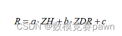
For more ideas, check out the business card below