Numerical solutions to second-order ordinary differential equations (central difference method and finite volume method)

Numerical solutions to second-order ordinary differential equations (central difference method and finite volume method)

Here we introduce the central difference method and the finite volume method to solve equations.
Question:
Use the central difference format of the difference method and the finite volume method to solve the two-point boundary value problem
$u^{\prime \prime }-a\left(2x-1\right)u^{\prime }-2o=0,0<x<1u\left(0\right)=u\left(1\right)=1,$
where parameter$a=10$ , the maximum error and convergence order of different grids are obtained.

problem analysis

Step 1: Mesh generation: First, take N + 1 nodes as: $a=x_0<x_1<x_2<\cdots <x_N=b$ ,
divide the interval [a, b] into equal intervals and divide it into N small intervals, note$h=x_{i+1}-x_i,i=1,2,\cdots ,N-1$ is the grid step size. Then perform dual decomposition: take adjacent nodes$x_{i+1},x_i$ 的中点$x_{i+\frac{1}{2}}=\frac{1}{2}\left(x_{i+1}-x_i\right),i=1,2,\cdots ,N-1.$ The analysis of the structure of the structure.
(i) Central difference method:
$\frac{1}{h^2}\left(u_{i+1}-2{and}_i+u_{i-1}\right)-\frac{\alpha \left(2x_i-1\right)}{2h\_}\left(u_{i+1}-u_{i-1}\right)-2\alpha u_i=0$
$\Rightarrow$
$\left(\frac{1}{h^2}-r_i\right)u_{i+1}+(-\frac{2}{h^2}-2a)\_u_i+\left(\frac{1}{h^2}+r_i\right)u_{i-1}=0$,

where $r_i=\frac{\alpha \left(2x_i-1\right)}{2h\_}.$
Let $A=\left[\begin{array}{cccccc}-\frac{2}{h^2}-2a& \frac{1}{h^2}-r_1& 0& \cdots & 0& 0\\ \frac{1}{h^2}+r_2& -\frac{2}{h^2}-2a& \frac{1}{h^2}-r_2& \cdots & 0& 0\\ \cdots & \cdots & \cdots & \cdots & \cdots & \cdots \\ 0& 0& 0& \cdots & \frac{1}{h^2}+r_{N-1}& -\frac{2}{h^2}-2\end{array}\right],$
$$\begin{gathered} U={\left(u_1,u_2,\cdots ,u_{N-1}\right)}^T, \\ b={\left(-u_0\left(\frac{1}{h^2}+r_1\right),0,0,\cdots ,0,-u_N\left(\frac{1}{h^2}+r_{N-1}\right)\right)}^T \end{gathered}$$ .
Then AU=b.
Then solve for U.

(ii) Finite volume method:
Let $W\left(x\right)=\frac{of}{dx}$, then $\frac{dW}{dx}-a\left(2x-1\right)W\left(x\right)-2o=0.$
两边同时积分得：
$W(x_{i+\frac{1}{2}})-W\left(x_{i-\frac{1}{2}}\right)-{\int }_{x_{i-\frac{1}{2}}}^{x_{i+\frac{1}{2}}}\alpha (2x-1)W(x)dx-{\int }_{x_{i-\frac{1}{2}}}^{x_{i+\frac{1}{2}}}2\alpha udx=0.$
运用积分中值定理可得：
$W(x_{i+\frac{1}{2}})-W\left(x_{i-\frac{1}{2}}\right)-W\left(x_i\right){\int }_{x_{i-\frac{1}{2}}}^{x_{i+\frac{1}{2}}}\alpha (2x-1)dx-u_i{\int }_{x_{i-\frac{1}{2}}}^{x_{i+\frac{1}{2}}}2\alpha dx=0.$
$\Rightarrow$
$W(x_{i+\frac{1}{2}})-W\left(x_{i-\frac{1}{2}}\right)-W(x_i)(x_{i+\frac{1}{2}}+x_{i-\frac{1}{2}}-1)h\alpha -2\alpha u_{i}h=0$
$\Rightarrow$
$\frac{1}{h}\left(u_{i+1}-2{and}_i+u_{i-1}\right)-\frac{}{4}\left(x_{i+1}+2x{\_}_i+x_{i-1}\right)\left(u_{i+1}-u_{i-1}\right)+\frac{}{2}\left(u_{i+1}-u_{i-1}\right)-{2\alpha u}_{i}h=0$
$\Rightarrow$
$\left(\frac{1}{h}-l_i+\frac{}{2}\right)u_{i+1}+\left(-\frac{2}{h}-2\alpha h\right)u_i+\left(\frac{1}{h}+l_i-\frac{}{2}\right)u_{i-1}=0,$
where$l_i=\frac{}{4}\left(x_{i+1}+2x{\_}_i+x_{i-1}\right)$ _
Let$A=\left[\begin{array}{cccccc}-\frac{2}{h}-2\alpha h& \frac{1}{h}-l_1+\frac{}{2}& 0& \cdots & 0& 0\\ \frac{1}{h}+l_2-\frac{}{2}& -\frac{2}{h}-2\alpha h& \frac{1}{h}-l_2+\frac{}{2}& \cdots & 0& 0\\ \cdots & \cdots & \cdots & \cdots & \cdots & \cdots \\ 0& 0& 0& \cdots & \frac{1}{h}+l_{N-1}-\frac{}{2}& -\frac{2}{h}-2\alpha \end{array}\right],$

$U={\left(u_1,u_1,\cdots ,u_{N-1}\right)}^T,F={\left(-u_0\left(\frac{1}{h}+l_1-\frac{}{2}\right),0,0,\cdots ,0,-u_N\left(\frac{1}{h}-l_{N-1}+\frac{}{2}\right)\right)}^T$
Then AU=F.
Then solve for U.

All codes are as follows (matlab)

function E=Centered(h)%中心差分法
u0=1;
uN=1;
N=1/h;
x=zeros(1,N+1);
for i=1:(N)
    x(i+1)=x(i)+h;
end
R=zeros(1,N+1);
for i=1:(N+1)
    R(i)=10*(2*x(i)-1)/(2*h);
end
A=zeros(N-1,N-1);
A(1,1)=-2/(h*h)-20;
A(1,2)=1/(h*h)-R(2);
A(N-1,N-1)=-2/(h*h)-20;
A(N-1,N-2)=1/(h*h)+R(N)
for i=2:(N-2)
        A(i,i)=-2/(h*h)-20;
        A(i,i+1)=1/(h*h)-R(i+1);
        A(i,i-1)=1/(h*h)+R(i+1);
end
b=zeros(1,N-1);
b(1)=-u0*(1/(h*h)+R(2));
b(N-1)=-uN*(1/(h*h)-R(N));
y=A\b';
Y=zeros(N+1,1);
Y(1,1)=1;
Y(N+1,1)=1;
for i=2:N
    Y(i,1)=y(i-1,1);
end
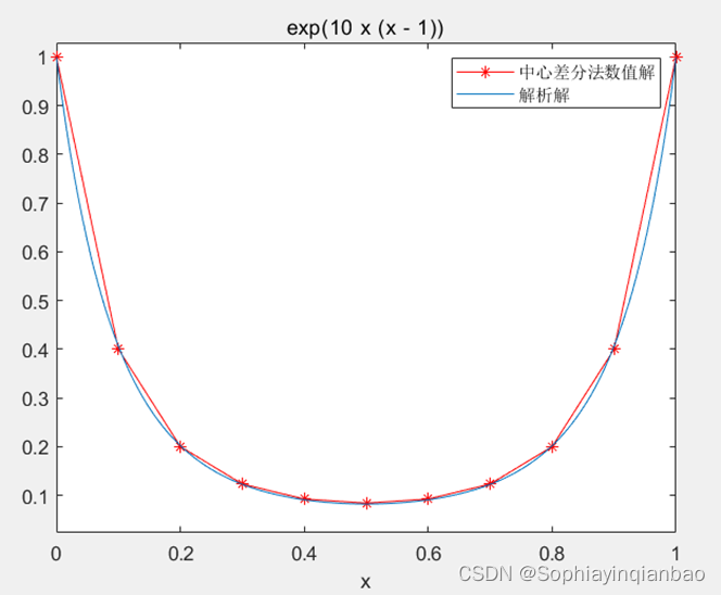
plot(x,Y ,'r*-');
hold on;
exa = dsolve('D2u = 10*(2*x-1)*Du+20*u', 'u(0)=1','u(1)=1', 'x');       %求出解析解
ezplot(exa, [0,1]);       %画出解析解的图像
legend('中心差分法数值解','解析解' );
u=zeros(1,N+1);
exa=inline(exa);
for i=1:(N+1)
    u(i)=feval(exa,x(i));
    e(i)=abs(u(i)-Y(i));
end
E=max(e);

function E=V(h)%有限体积法
u0=1;
uN=1;
N=1/h;
x=zeros(1,N+1);
for i=1:(N)
    x(i+1)=x(i)+h;
end
R=zeros(1,N+1);
for i=2:N
    R(i)=2.5*(x(i+1)+2*x(i)+x(i-1));
end
A=zeros(N-1,N-1);
A(1,1)=-2/h-20*h;
A(1,2)=1/h+5-R(2);
A(N-1,N-1)=-2/h-20*h;
A(N-1,N-2)=1/h-5+R(N);
for i=2:(N-2)
        A(i,i)=-2/h-20*h;
        A(i,i+1)=1/h+5-R(i+1);
        A(i,i-1)=1/h-5+R(i+1);
end
b=zeros(1,N-1);
b(1)=-u0*(1/h-5+R(2));
b(N-1)=-uN*(1/h+5-R(N));
y=A^(-1)*b';
Y=zeros(N+1,1);
Y(1,1)=1;
Y(N+1,1)=1;
for i=2:N
    Y(i,1)=y(i-1,1);
end
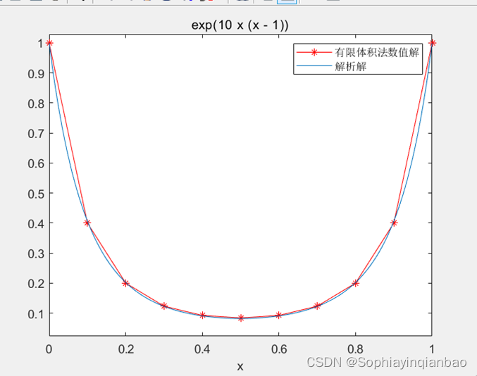
plot(x,Y ,'r*-');
hold on;
exa = dsolve('D2u = 10*(2*x-1)*Du+20*u', 'u(0)=1','u(1)=1', 'x');       %求出解析解
ezplot(exa, [0,1]);       %画出解析解的图像
legend('有限体积法数值解','解析解' );
u=zeros(1,N+1);
exa=inline(exa);
for i=1:(N+1)
    u(i)=feval(exa,x(i));
    e(i)=abs(u(i)-Y(i));
end
E=max(e);
%调试
clear all;clc;close  all;
h=[0.1,0.2,0.01,0.02,0.05];
for i=1:5
    E(i)=V(h(i));
    F(i)=Centered(h(i));
end

Question result

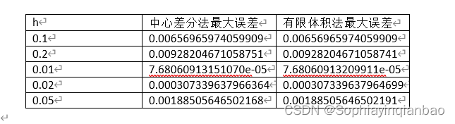
We found that the maximum error of the central difference method and the finite volume method have a small difference and the order is the same. Therefore, we can think that the convergence orders of the central difference method and the finite volume method are the same, and we know that the convergence of the central difference method is the same. The order is 2nd order, so the convergence order of the finite volume method is also 2nd order.

(Taking h=0.1 as an example, we drew the images of the numerical solution and the analytical solution of the two methods)