YOLO v2
Compared with yolo v1, the updates of yolo v2 are mainly reflected in the following aspects: the update of the backbone network , the introduction of the anchor mechanism, and some small details such as global avgpooling , the passthrough structure similar to FPN in v3 , and the BN layer is used and abandoned. dropout and so on.
1. Update of the backbone network.
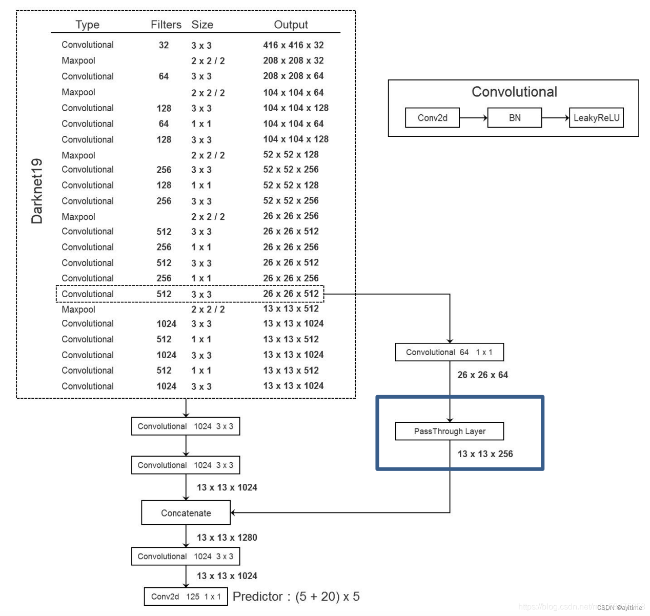
Darknet19 is used instead of the original vgg16. The mAP is basically unchanged but the number of parameters is reduced, thereby increasing the speed of training and prediction. I think the main contribution is to achieve dimensionality reduction in the channel direction (compression of the tensor) by introducing 1×1 convolution to compress the parameter amount. After the dimensionality reduction of the tensor, the features are extracted through normal 3×3 convolution and the dimension is raised again. . (Similar to the BottleNeck bottleneck structure in ResNet)
Structural comparison of the two networks:
 vgg16
vgg16
|
 Darknet19 Darknet19
|
At the same time, dropout was abandoned; a BN layer (normal distribution nb) was added after the convolutional layer to squeeze the output of each layer near 0 to prevent the output of each layer of neurons from being too far away from 0 and causing the gradient to disappear and prevent over-fitting. combine.
2. Introducing the anchor mechanism
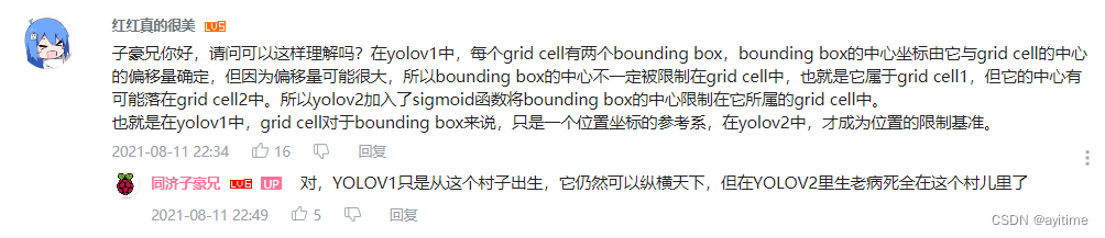
in yolo v1, which of the two bounding boxes of each grid cell is responsible for predicting the object is uncertain, and the shape wh is also randomly predicted. There is no limit to running the whole picture, and it is difficult to train. The anchor mechanism introduced in yolo v2, each grid cell has five anchor sizes, and the bbox is fine-tuned based on the anchor prediction results (obtained in advance by k-means on the data set based on the image size); quite Make key points before the exam so that candidates are familiar with what will be tested in the exam).
The anchor can also be called the prior bounding box "prior box" or the anchor box "anchor box", which will be collectively referred to as anchor in the future; the
box after the anchor is adjusted according to the prediction result, that is, the prediction box is called "bounding box", or bbox for short (see 3 for how to adjust) ).
Anchor matching principle: If the center of the gt frame falls in a certain grid, calculate the anchor with the largest iou of the gt frame among the five anchors in the grid as the frame to predict the object. If another GT also falls into the grid and matches an anchor of another size, then this anchor will be responsible for predicting the GT (that is, all five anchors of a grid can predict objects at the same time, which is the same as a grid in yolo v1 Only one of the two bboxes is responsible for predicting different objects!!)
After selecting the box, the model is fine-tuned into a bbox based on this anchor, and hopes to be adjusted into the xywh of gt

In addition, the introduction of the anchor mechanism can help the network learn more easily , so the FC layer that was previously responsible for prediction can be removed and replaced with the bottom 1×1 convolution in the picture above to achieve prediction (very happy!)
In addition, I attach an answer from brother Tongji Zihao to deepen my understanding:
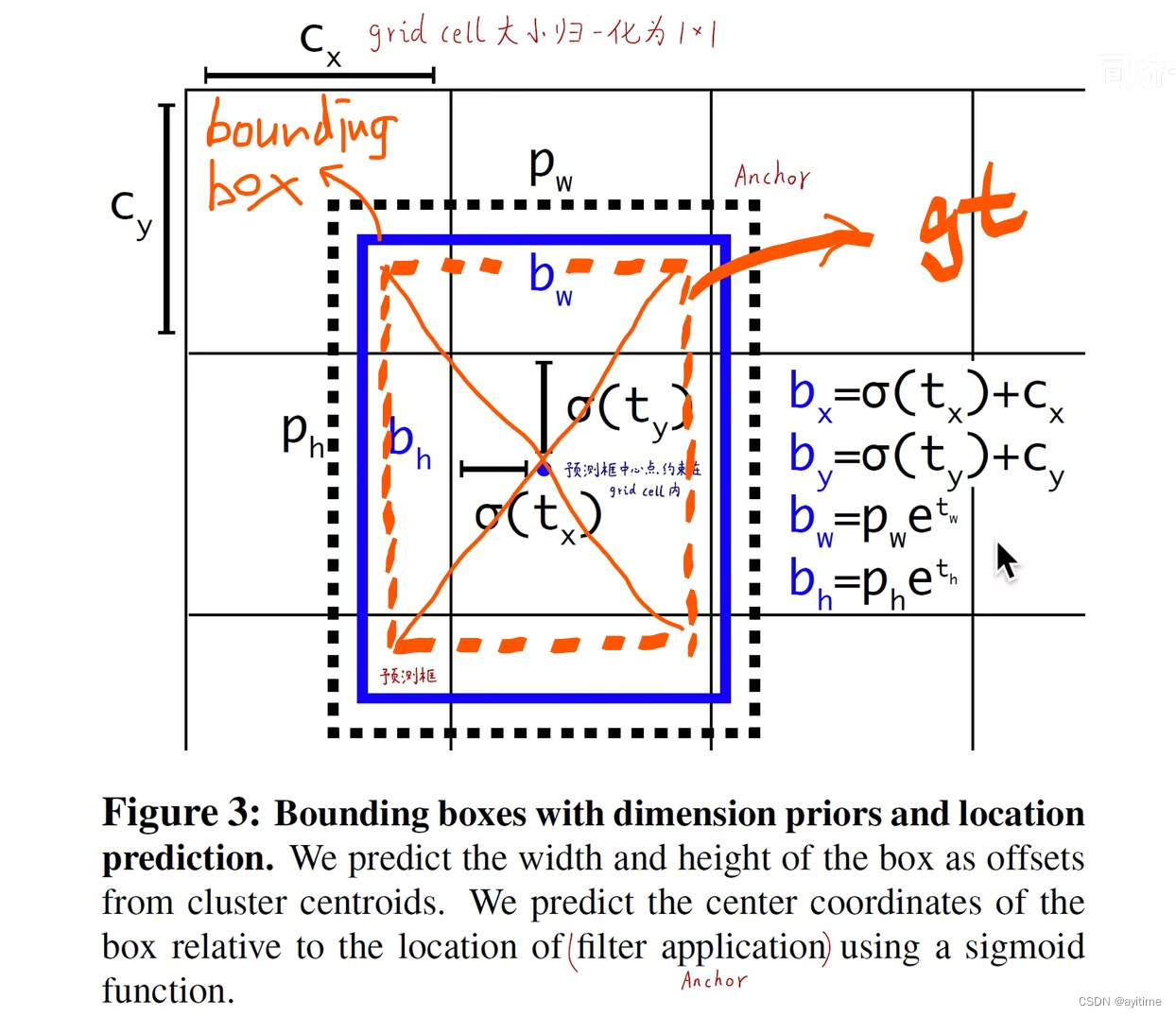
3. Direct location prediction (absolute location prediction)
is directly shown in the picture above. You can only understand it by looking at the post without looking at the code. One thing to be clear in advance: anchor only has the shape attribute of wh, but no xy position attribute. The following introduces the testing process first and then introduces the training process in turn:
Prediction process :
The grid predicted by the model predicts 5 groups of tx ty tw th, and the sizes of the 5 anchors are calculated according to the formula in the figure below. The final prediction frame xywh can be obtained, and then After the subsequent nms...balabala...
training process :
First, the center of the gt box must fall in the grid, as shown by the orange dotted line in the figure; how do we select the anchor? Align the five anchors with the center of the gt frame, and select the one with the largest iou, which is the outermost black dotted line in the picture.
Afterwards, we need to adjust the position and size of the anchor: we want to adjust the center of the anchor to the center of the gt box, and because the center of the anchor must fall within the grid, and the position of the upper left corner of the grid is known (according to gt ), so it can be achieved by predicting the normalized offset relative to the upper left corner of the grid, which is equivalent to letting the network return a floating point number between 0 and 1 , implemented through sigmoid (reducing sensitivity).
The adjustment of w and h is based on the width and height of the anchor. The direct difference in yolo v1 is converted into the size change rate, that is, the network is allowed to return a floating point number near 1 , and the logarithm e is used to achieve it (reduce sensitivity).
4. Changes in loss after introducing anchor.
The loss adds the above two parts based on v1:
- The first line:
Confidence error for prediction box and gt box iou<0.6 (how to calculate it, all bbox and gt are calculated for iou???). The corresponding background of such boxes should make them not responsible for predicting objects, that is, the confidence level is 0; - Second line:
How to make each grid cell of the network generate a bounding box (shape) near the anchor (shape)? In the early stage of network training (epoch<12800), the predicted bbox shape is restricted (? proir itself should not With position xy information, is it possible to move the anchor to the center of the gt box, and then calculate the position deviation between the anchor at this time and the predicted bbox (anchor + offset)? To be confirmed) - The following is basically the same as v1, for the three-part loss of the prediction box responsible for predicting the object.
In fact, prediction boxes can be divided into three types, corresponding to poor students, average students, and top students; poor students are bboxes whose iou of bbox and gt are less than 0.6, top students are bboxes responsible for predicting objects, and the rest are average students. Only poor students (background) and Top students (predicting the bbox of the object) participate in the loss calculation, while average students do not. (I’m not sure about the definition of poor students, I need to confirm it after comparing it with v3)

5. Use of pass through
In the right branch in the darknet19 figure, the underlying fine-grained and high-level semantic features are fused. The same principle as v3's FPN: it retains deep semantic information and integrates shallow location information.
6. global avgpooling
global average pooling (in the channel direction) to achieve input of any size and replaces FC.
Posts on the Internet are all like this. I looked for several models and couldn’t see where this GAP is used. If anyone is more pragmatic, please let me know.