Table of contents
- 1. Learning points
- 2. Definition of algorithm
- 3. Nature of algorithm
- 4. Program
- 5. Problem Solving
- 6. Description of algorithm
- 7. The purpose of algorithm analysis
- 8. Algorithm complexity analysis
-
- (1) Algorithm time complexity analysis
- (2) Asymptotic complexity of algorithm
-
- 1. Asymptotic upper bound notation-Big O notation
- 2. Asymptotic lower bound notation-big Ω symbol
- 3. Compact asymptotic notation-Θ symbol
- 4. Non-tight upper bound symbol o
- 5. Non-compact lower bound symbol ω
- 6. The significance of asymptotic analysis notation in equations and inequalities
- 7. Comparison of functions in asymptotic analysis
- 8. Some properties of asymptotic analysis symbols
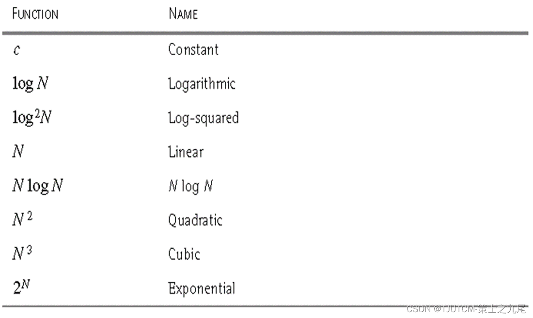
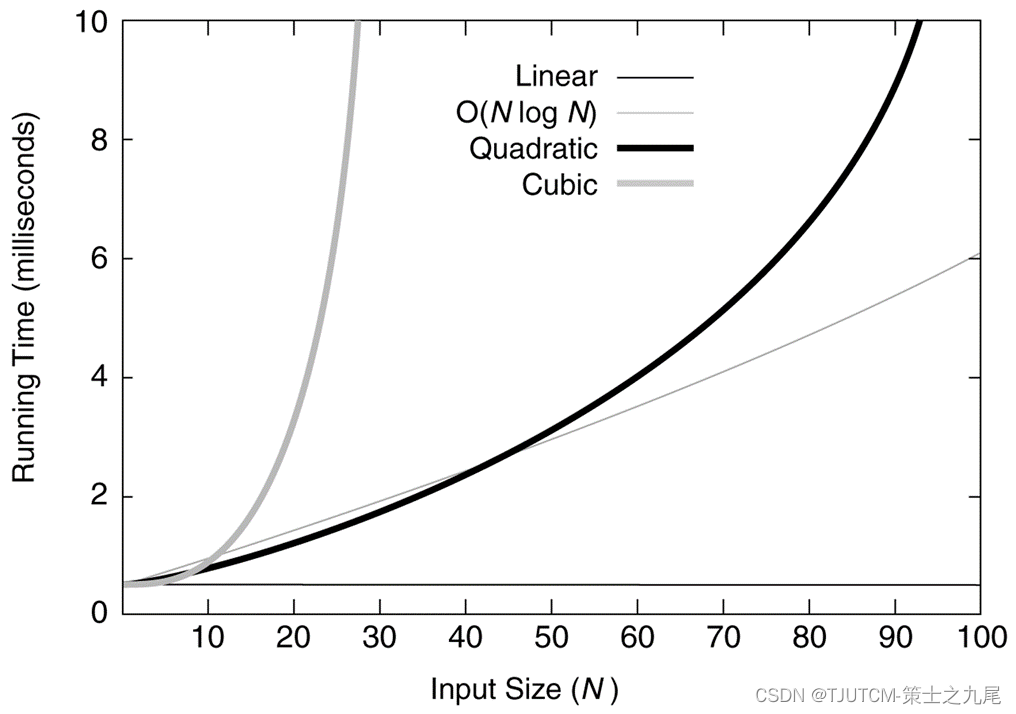
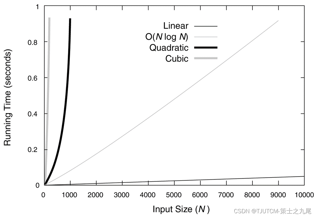
- 9. Commonly used functions in algorithm asymptotic complexity analysis
- 10. Common complexity functions in algorithm analysis
- 9. Basic rules of algorithm analysis
Data structure + algorithm (+ design pattern) = program
1. Learning points
Understand the concept of algorithms.
Master the concept of computational complexity of algorithms.
Master the mathematical expression of the asymptotic behavior of algorithmic complexity.
Understand the basic concepts of NP problems.
2. Definition of algorithm
As the name suggests, the calculation (solution) method
algorithm (Algorithm): a description of the steps to solve a specific problem, is a limited sequence of instructions .
An algorithm refers to a method or process for solving a problem .
Programming = data structure + algorithm (+ design pattern)
3. Nature of algorithm
An algorithm is a finite sequence of several instructions that satisfies the following properties:
(1) Input : There are externally provided quantities as inputs to the algorithm.
(2) Output : The algorithm produces at least one quantity as output.
(3) Determinism : Each instruction that makes up the algorithm is clear and unambiguous.
(4) Finiteness : The number of executions of each instruction in the algorithm is limited, and the time to execute each instruction is also limited.
4. Program
A program is the specific implementation of an algorithm in a certain programming language.
The program does not need to satisfy the properties of the algorithm.
An operating system, for example , is a program that executes in an infinite loop, and is therefore not an algorithm .
The various tasks of the operating system can be regarded as separate problems , and each problem is implemented by a subroutine in the operating system through a specific algorithm . The subroutine terminates after getting the output result.
5. Problem Solving
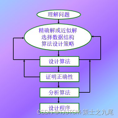
6. Description of algorithm
Natural language or tabular
pseudocode method
C++ language
Java language
C language
Python and other languages
7. The purpose of algorithm analysis
Estimate the two computer resources required by the algorithm - time and space. Design
algorithm - design an algorithm with the lowest possible complexity.
Select algorithm - choose the least complex algorithm among multiple algorithms.
8. Algorithm complexity analysis
Algorithm complexity is the amount of computer resources required to run an algorithm.
The amount of time resources required is called time complexity , and the amount of space resources required is called space complexity .
This quantity should depend only on the size of the problem the algorithm is trying to solve , the inputs to the algorithm , and a function of the algorithm itself .
If N , I and A are used to represent the scale of the problem to be solved by the algorithm , the input of the algorithm and the algorithm itself , and C is used to represent the complexity, then there should be C=F(N,I,A) .
Generally, time complexity and space complexity are separated and represented by T and S respectively, then there are: T=T(N,I) and S=S(N,I) (usually, let A be implicit in the complexity function name)
(1) Algorithm time complexity analysis
Worst-case time complexity :

Best-case time complexity :

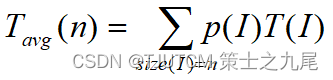
Average-case time complexity :
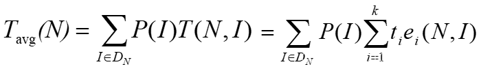
where DN is a set of legal inputs of size N; I* is DN such that T(N, I* ) reaches Tmax(N); is the legal input that makes T(N, I*) reach Tmin(N); and P(I) is the probability of input I appearing in the application of the algorithm.
(2) Asymptotic complexity of algorithm
T(n) →∞ , when n→∞ ;
(T(n) - t(n) )/ T(n) →0 , when n→∞;
t(n) is the asymptotic behavior of T(n) , is the asymptotic complexity of the algorithm.
Mathematically, t(n) is the asymptotic expression of T(n), which is the main term left by T(n) omitting the low-order terms. It is simpler than T(n).
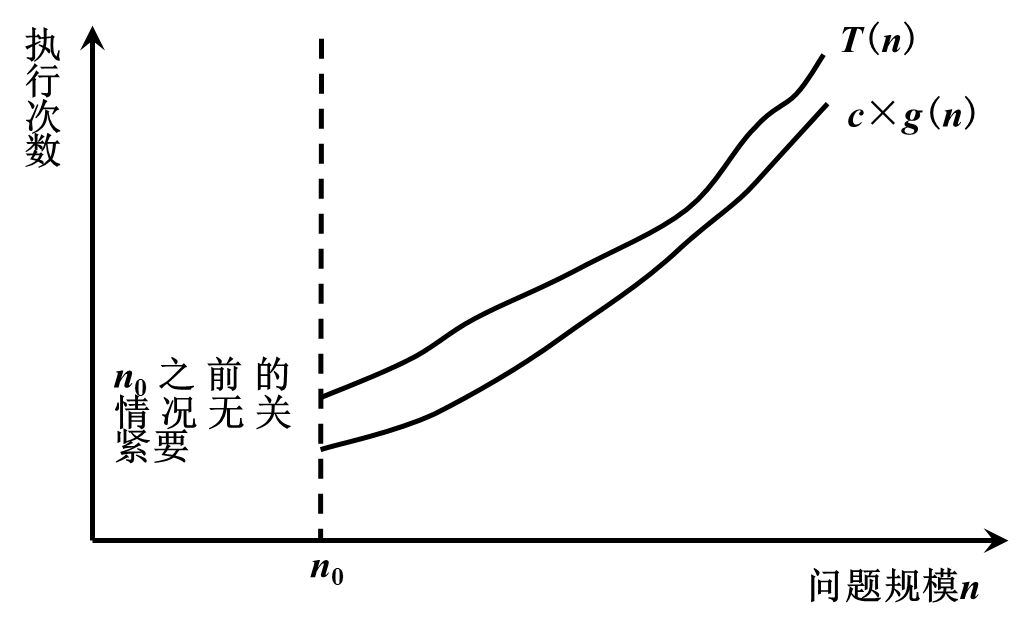
1. Asymptotic upper bound notation-Big O notation
If there are two positive constants c and n0, and for any n≥n0, there is T(n)≤c×f(n), then it is said that T(n)=O(f(n))

2. Asymptotic lower bound notation-big Ω symbol
If there are two positive constants c and n0, and for any n≥n0, there is T(n)≥c×g(n), then it is said that T(n)=Ω(g(n))
3. Compact asymptotic notation-Θ symbol
If there are three positive constants c1, c2 and n0, and for any n≥n0, c1×f(n)≥T(n)≥c2×f(n), it is said that T( n)=Θ(f( n))

Example: T(n)=5n2+8n+1
When n≥1, 5n2+8n+1≤5n2+8n+n=5n2+9n≤5n2+9n2≤14n2=O(n2)
When n≥1, 5n2+8n+1≥5n2=Ω(n2)
∴ When n≥1 When, 14n2≥5n2+8n+1≥5n2
then: 5n2+8n+1=Θ(n2)
Theorem: If T(n)=amnm +am-1nm-1 + … +a1n+a0 (am>0), then T(n)=O (nm) and T(n)=Ω(nm), therefore, T(n)=Θ(nm).
4. Non-tight upper bound symbol o
o(g(n)) = { f(n) | For any positive constant c>0, there is a positive number and n0 >0 such that for all n≥n0: 0<f(n)<cg(n) }
etc. Valence is f(n) / g(n) →0 when n→∞.
5. Non-compact lower bound symbol ω
ω(g(n)) = { f(n) | For any positive constant c>0, there exists a positive sum n0 >0 such that for all n> n0: 0 ≤ cg(n) < f(n) }
etc. Valence is f(n) / g(n) →∞, when n→∞.
6. The significance of asymptotic analysis notation in equations and inequalities
The exact meaning of f(n)= Θ(g(n)) is: f(n) ∈ Θ(g(n)).
In general, the asymptotic notation Θ(g(n)) in equations and inequalities represents a function in Θ(g(n)).
For example: 2n2 + 3n + 1 = 2n2 + Θ(n) means
2n2 +3n +1=2n2 + f(n), where f(n) is a function in Θ(n).
The meanings of the asymptotic symbols O, o, Ω and ω in equations and inequalities are similar.
7. Comparison of functions in asymptotic analysis
f(n)= O(g(n)) ≈ a ≤ b;
f(n)= Ω(g(n)) ≈ a ≥ b;
f(n)= Θ(g(n)) ≈ a = b;
f(n)= o(g(n)) ≈ a < b;
f(n)= ω(g(n)) ≈ a > b.
8. Some properties of asymptotic analysis symbols
(1) Transitivity
f(n)= Θ(g(n)), g(n)= Θ(h(n)) → f(n)= Θ(h(n)); f(n)= O(g(n
) ), g(n)= O (h(n)) → f(n)= O (h(n));
f(n)= Ω(g(n)), g(n)= Ω (h( n)) → f(n)= Ω(h(n));
f(n)= o(g(n)), g(n)= o(h(n)) → f(n)= o( h(n));
f(n)= ω(g(n)),g(n)= ω(h(n)) → f(n)= ω(h(n));
(2) Reflexivity
f(n)= Θ(f(n));
f(n)= O(f(n));
f(n)= ω(f(n)).
(3) Symmetry
f(n)= Θ(g(n)) ⇔ g(n)= Θ (f(n)) .
(4) Mutual symmetry
f(n)= O(g(n)) ⇔ g(n)= Ω (f(n)) ;
f(n)= o(g(n)) ⇔ g(n)= ω (f(n) ) ;
(5) Arithmetic operations
O(f(n))+O(g(n)) = O(max{f(n),g(n)}) ;
O(f(n))+O(g(n)) = O(f(n)+g(n)) ;
O(f(n))*O(g(n)) = O(f(n)*g(n)) ;
O(cf(n)) = O(f(n)) ;
g(n)= O(f(n)) → O(f(n))+O(g(n)) = O(f(n)) 。
Rule O(f(n))+O(g(n)) = O(max{f(n),g(n)})prove:
For any f1(n) ∈ O(f(n)), there is a positive constant c1 and a natural number n1 such that f1(n) ≤ c1f(n) for all n≥ n1.
Similarly, for any g1(n) ∈ O(g(n)) , there are positive constants c2 and natural numbers n2 such that g1(n) ≤ c2g(n) for all n≥ n2.
Let c3=max{c1, c2}, n3 =max{n1, n2}, h(n)= max{f(n),g(n)}.
Then for all n ≥ n3,
f1(n) +g1(n) ≤ c1f(n) + c2g(n)
≤ c3f(n) + c3g(n)= c3(f(n) + g(n) )
≤ c32 max{f(n),g(n)}
= 2c3h(n) = O(max{f(n),g(n)}) .
9. Commonly used functions in algorithm asymptotic complexity analysis
(1) Monotone function
Monotonically increasing : m ≤ n → f(m) ≤ f(n);
Monotonically decreasing : m ≥ n → f(m) ≥ f(n);
Strict monotonic increasing : m < n → f(m) < f(n );
strictly monotonically decreasing : m > n → f(m) > f(n).
(2) Rounding function
⌊ x ⌋: the largest integer not greater than x ;
⌈ x ⌉: the smallest integer not less than x .
Some properties of rounding functions
x-1 < ⌊ x ⌋ ≤ x ≤ ⌈ x ⌉ < x+1;
⌊ n/2 ⌋ + ⌈ n/2 ⌉ = integer n;
for n ≥ 0, a,b>0, there is:
⌈ ⌈ n/ a ⌉ /b ⌉ = ⌈ n/ab ⌉ ;
⌊ ⌊ n/a ⌋ /b ⌋ = ⌊ n/ab ⌋ ;
⌈ a/b ⌉ ≤ (a+(b-1))/b;
⌊ a/b ⌋ ≥ (a-(b-1))/b;
f(x)= ⌊ x ⌋ , g(x)= ⌈ x ⌉ are monotonically increasing functions.
(3)Polynomial function
p(n)= a0+a1n+a2n2+...+adnd> ad>0;
p(n) = Θ(nd);
f(n) = O(nk) ⇔ f(n) is infinitesimal:
f(n) = O(1) ⇔ f(n) ≤ c;
k ≥ d → p(n) = O(nk);
k ≤ d → p(n) = Ω(nk);
k > d → p(n) = o(nk);
k < d → p(n) = ω(nk)
(4) Exponential function
For positive integers m,n and real numbers a>0:
a0=1;
a1=a;
a-1=1/a;
(am)n = amn;
(am)n = (an)m;
aman = am+n ;
a>1 → an is a monotonically increasing function;
a>1 →
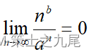
→ nb = o(an)
(5) Logarithmic function
log n = log2n;
lg n = log10n;
ln n = logen;
logkn = (log n)k;
log log n = log(log n);
for a>0,b>0,c>0

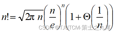
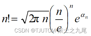
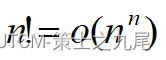
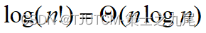
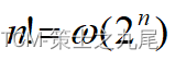
(6) Factorial function
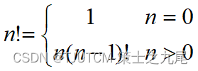
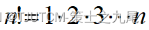
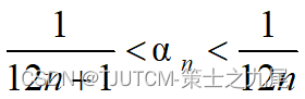
Stirling’s approximation
10. Common complexity functions in algorithm analysis
(1) Small-scale data
(2) Medium-sized data
(3) Algorithm analysis method
Example: Sequential search algorithm
template<class Type>
int seqSearch(Type *a, int n, Type k)
{


     for(int i=0;i<n;i++)
	  if (a[i]==k) return i;
     return -1;
}
(1) Tmax(n) = max{ T(I) | size(I)=n }=O(n) (
2) Tmin(n) = min { T(I) | size(I)=n }= O(1)
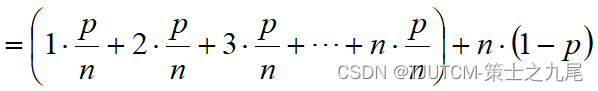
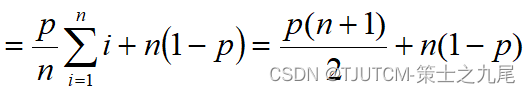
(3) Under average circumstances, assume:
(a) The probability of successful search is p (0 ≤ p ≤ 1);
(b) The search is successful at each position i (0 ≤ i < n) of the array The probabilities are the same, both are p/n.
9. Basic rules of algorithm analysis
1. Non-recursive algorithm:
(1) for / while loop
The calculation time in the cycle body * the number of cycles ;
(2) Nested loops
Cycle body calculation time * all cycle times ;
(3) Sequential statements
The calculation time of each statement is added together ;
(4) if-else statement
The larger of the if statement calculation time and the else statement calculation time .
2. Optimal algorithm
The lower bound of the calculation time of the problem is Ω(f(n)), then the algorithm with the calculation time complexity of O(f(n)) is the optimal algorithm.
For example, the lower bound of the calculation time of the sorting problem is Ω(nlogn), and the sorting algorithm with a computational time complexity of O(nlogn) is the optimal algorithm.
Heap sort algorithm is the optimal algorithm.