[Deep Learning Experiment] Linear Model (4): Using Pytorch to implement a linear model: Using stochastic gradient descent optimizer to train the model

Table of contents

1. Experiment introduction

2. Experimental environment

1. Configure the virtual environment

2. Library version introduction

3. Experimental content

0. Import library

1. Linear model linear_model

2. Loss function loss_function

3. Define data

4. Initialize weights and biases

5. Model training

6. Iteration

7. Experimental results

8. Complete code

---

1. Experiment introduction

        Train a linear model using a stochastic gradient descent optimizer and output the optimized parameters

 2. Experimental environment

        This series of experiments uses the PyTorch deep learning framework. The relevant operations are as follows:

1. Configure the virtual environment

conda create -n DL python=3.7 

conda activate DL

pip install torch==1.8.1+cu102 torchvision==0.9.1+cu102 torchaudio==0.8.1 -f https://download.pytorch.org/whl/torch_stable.html

conda install matplotlib

 conda install scikit-learn

2. Library version introduction

software package	This experimental version	The latest version currently
matplotlib	3.5.3	3.8.0
numpy	1.21.6	1.26.0
python	3.7.16
scikit-learn	0.22.1	1.3.0
torch	1.8.1+cu102	2.0.1
torchaudio	0.8.1	2.0.2
torchvision	0.9.1+cu102	0.15.2

3. Experimental content

ChatGPT：

         Stochastic Gradient Descent (SGD) is a commonly used optimization algorithm for training machine learning models. It is a variant of the gradient descent algorithm and is mainly used in the case of large-scale data sets or high-dimensional parameter spaces.

        The goal of the gradient descent algorithm is to find the optimal solution to the model parameters by minimizing the loss function. In the traditional gradient descent algorithm, each training cycle (epoch) needs to calculate the gradient of the entire training set and then update the model parameters. This approach is computationally expensive on large-scale datasets because each training cycle requires traversing the entire dataset.

        Unlike traditional gradient descent, stochastic gradient descent uses only one sample (or a small batch of samples) per iteration to calculate the gradient and update the model parameters. Specific steps are as follows:

1. Initialize model parameters.
2. Randomly shuffle the training data set.
3. For each training sample (or mini-batch):
   • Calculate the model's predicted value for the current sample.
   • Calculate the gradient of the loss function for the current sample.
   • Update model parameters based on gradient and learning rate.
4. Repeat step 3 until the predetermined number of training cycles is reached or the stopping condition is met.

        The main advantage of stochastic gradient descent is that it is computationally efficient, especially for large-scale data sets. It also performs parameter updates in every training epoch, so it converges faster. However, since only one sample (or mini-batch of samples) is used per iteration, the update direction of stochastic gradient descent may be more unstable, causing the loss function to fluctuate during training. To alleviate this problem, techniques such as learning rate decay and momentum can be used to improve the algorithm.

This series is experimental content and does not explain theoretical knowledge in detail.

(Ahem, I actually don’t have time to sort it out. I’ll come back and fill in the gaps when I have the opportunity)

0. Import library

import torch

1. Linear modellinear_model

        This function accepts input data x, uses randomly generated weights wand biases b, and calculates an output value output. The form of the linear model here is  output = x * w + b.

def linear_model(x):
    return torch.matmul(x, w) + b

2. Loss functionloss_function

      The mean square error (MSE) is used here as the loss function to calculate the square of the difference between the predicted value and the true value.

def loss_function(y_true, y_pred):
    loss = (y_pred - y_true) ** 2
    return loss

3. Define data

• Generate a random input tensor  xwith a shape of (5, 1), indicating that there are 5 samples and the feature dimension of each sample is 1.

• Generate a target tensor  ywith shape (5, 1), representing the corresponding true label.

• Prints information about the data, including input xand target values ​​for each sample y.

x = torch.rand(5, 1)
y = torch.tensor([1, -1, 1, -1, 1], dtype=torch.float32).view(-1, 1)
print("The data is as follows:")
for i in range(x.shape[0]):
    print("Item " + str(i), "x:", x[i][0], "y:", y[i])

4. Initialize weights and biases

w = torch.rand(1, 1, requires_grad=True)
b = torch.randn(1, requires_grad=True)

5. Model training

model = linear_model(x, w, b)
optimizer = optim.SGD([w, b], lr=0.01)  # 使用SGD优化器

6. Iteration

num_epochs = 100  # 迭代次数
for epoch in range(num_epochs):
    optimizer.zero_grad()   # 梯度清零
    prediction = linear_model(x, w, b)
    loss = loss_function(y, prediction)
    loss.mean().backward()  # 计算梯度
    optimizer.step()        # 更新参数
    # print(w, b)
    if (epoch + 1) % 10 == 0:
        print(f"Epoch {epoch + 1}/{num_epochs}, Loss: {loss.mean().item()}")

• In each iteration:

  • Clear the optimizer's gradient cache to zero, and then use the current weights and biases to  x predict the input to get the prediction result  prediction.

  • The loss tensor is obtained by  loss_function calculating the loss between the predicted result and the true label  loss.

  • Call to  loss.mean().backward() calculate the average of the loss and perform backpropagation based on the calculated gradient.

  • Call  optimizer.step() update weights and biases, using the optimizer for gradient descent updates.

  • Every 10 iterations, the sequence number of the current iteration, the total number of iterations, and the average loss are output.

7. Experimental results

print("The optimized parameters are:")
print("w:", model[0].item())
print("b:", model[1].item())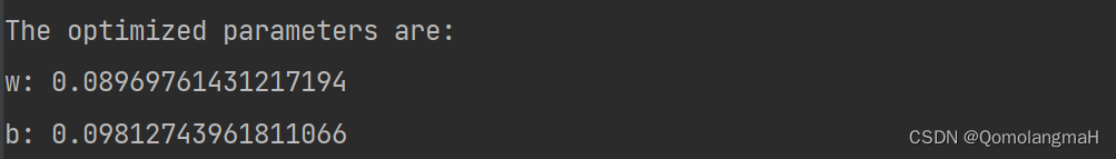

8. Complete code

import torch
import torch.optim as optim


def linear_model(x, w, b):
    return torch.matmul(x, w) + b


def loss_function(y_true, y_pred):
    loss = (y_pred - y_true) ** 2
    return loss


x = torch.rand(5, 1)
y = torch.tensor([1, -1, 1, -1, 1], dtype=torch.float32).view(-1, 1)
print("The data is as follows:")
for i in range(x.shape[0]):
    print("Item " + str(i), "x:", x[i][0], "y:", y[i])

w = torch.rand(1, 1, requires_grad=True)
b = torch.randn(1, requires_grad=True)
model = linear_model(x, w, b)
optimizer = optim.SGD([w, b], lr=0.01)  # 使用SGD优化器

num_epochs = 100  # 迭代次数
for epoch in range(num_epochs):
    optimizer.zero_grad()   # 梯度清零
    prediction = linear_model(x, w, b)
    loss = loss_function(y, prediction)
    loss.mean().backward()  # 计算梯度
    optimizer.step()        # 更新参数
    # print(w, b)
    if (epoch + 1) % 10 == 0:
        print(f"Epoch {epoch + 1}/{num_epochs}, Loss: {loss.mean().item()}")

print("The optimized parameters are:")
print("w:", model[0].item())
print("b:", model[1].item())

Notice:

        This experiment uses randomly generated data, so training does not make any sense. The following will be based on the classic iris data set to conduct experiments and evaluate the model.