[Click] Join the large model technology exchange group
In recent years, with the introduction of Transformer and MOE architectures, deep learning models have easily exceeded trillions of scale parameters. The traditional single-machine single-card model can no longer meet the requirements for training extremely large models. Therefore, we need to train distributed large models based on multiple cards on a single machine or even on multiple machines and cards.
The primary goal of distributed machine learning is to use AI clusters to enable deep learning algorithms to better efficiently train large models with excellent performance from large amounts of data. In order to achieve this goal, it is generally necessary to consider dividing the computing tasks, training data and models according to the matching of hardware resources and data/model scale, so as to carry out distributed storage and distributed training. Therefore, distributed training related technologies deserve our in-depth analysis of the mechanisms behind them.
The following mainly explains the parallel technology for distributed training of large models. This series is roughly divided into eight articles.
Large model distributed training parallel technology (1) - overview
Large model distributed training parallel technology (2) - data parallelism
Large model distributed training parallel technology (3) - pipeline parallelism
Large model distributed training parallel technology (4) - tensor parallelism
Large model distributed training parallel technology (5) - sequence parallelism
Large model distributed training parallel technology (6) - multi-dimensional hybrid parallelism
Large model distributed training parallel technology (7)-automatic parallelism
Large model distributed training parallel technology (8)-MOE parallelism
In the previous article, data parallel training, an obvious feature is that each GPU holds a copy of the entire model weights, which brings about redundancy problems. Although FSDP can alleviate the redundancy problem, for very large-scale models Generally speaking, only using data parallelism for distributed training cannot further increase the parameter scale of the model. Therefore, the text tells that another parallelization technique is model parallelism, that is, the model is divided and distributed on an array of devices, and each device only saves a part of the parameters of the model.
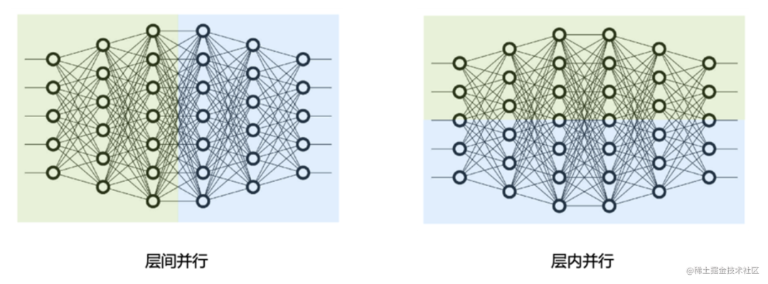
Model parallelism is divided into tensor parallelism and pipeline parallelism. Tensor parallelism is intra-layer parallelism, which divides the model Transformer layer. The pipeline is inter-layer parallelism, which divides different Transformer layers of the model.
This article is the third article of distributed training parallel technology: pipeline parallelism. The following will mainly describe the common pipeline parallel methods GPipe and PipeDream and their variants in the industry.
Introduction
The so-called pipeline parallelism means that because the model is too large, the entire model cannot be placed on a single GPU card; therefore, different layers of the model are placed on different computing devices to reduce the memory consumption of a single computing device, thereby achieving ultra-large-scale model training .
As shown in the figure below, the model contains a total of four model layers (such as the Transformer layer), which are divided into three parts and placed on three different computing devices. That is, the first layer is placed on device 0, the second and third layers are placed on device 1, and the fourth layer is placed on device 2.
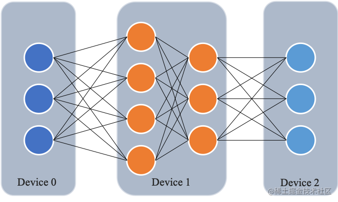
Data is transmitted between adjacent devices through communication links. Specifically, during the forward calculation process, the input data is first calculated on layer 1 on device 0 to obtain the intermediate result, and the intermediate result is transmitted to device 1, and then calculated on device 1 to obtain layer 2 and layer 3. The output of the third layer of the model is transmitted to device 2, and the forward calculation result is obtained through the calculation of the last layer on device 2. The backpropagation process is similar. Finally, the network layers on each device update their parameters using the gradients calculated by the backpropagation process. Since only the output tensors between adjacent devices are transmitted between each device instead of gradient information, the communication volume is small.
Naive pipeline parallelism
Naive pipeline parallelism is the most direct method to achieve pipeline parallel training. We divide the model into multiple parts (Stage) according to the layers, and assign each part (Stage) to a GPU. We then perform regular training on mini-batches of data, communicating at the boundaries where the model is split into parts.
The following takes the 4-layer sequential model as an example:
output=L4(L3(L2(L1(input))))We distribute the computation to two GPUs as follows:
GPU1 computes:
intermediate=L2(L1(input))GPU2 computes:
output=L4(L3(intermediate))
To complete the forward pass, we compute the intermediate values on GPU1 and transfer the resulting tensor to GPU2. GPU2 then computes the model's output and begins backpropagation. For backpropagation, we send gradients halfway from GPU2 to GPU1. Then, GPU1 completes backpropagation based on the sent gradients. This way, pipelined parallel training produces the same outputs and gradients as single-node training. Naive pipeline parallel training is equivalent to sequential training, which makes debugging easier.
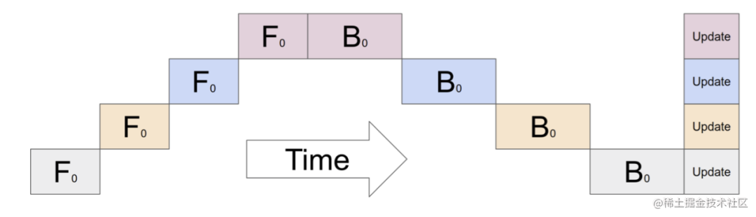
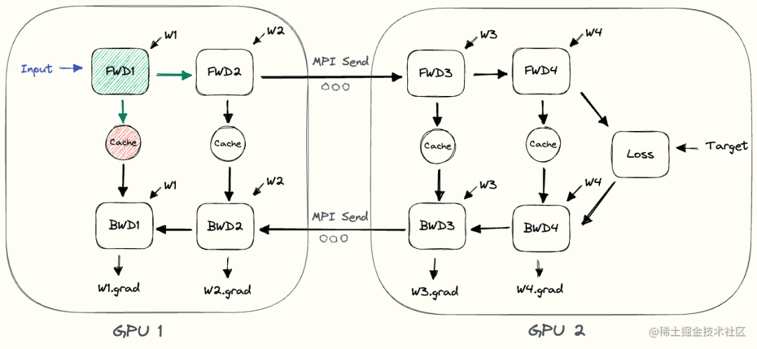
The following illustrates the naive pipeline parallel execution process. GPU1 performs forward pass and caches activations (red). It then sends the output of L2 to GPU2 using MPI. GPU2 completes the forward pass and uses the target value to calculate the loss, and then starts the back pass. Once GPU2 completes, the output of the gradient is sent to GPU1, thus completing backpropagation.
Note that only point-to-point communication (MPI.Send and MPI.Recv) is used here, and no collective communication primitives are required (thus, no MPI.AllReduce is required).
Problems with naive pipeline parallelism :
So why is this method called naive pipeline parallelism, and what are its shortcomings?
Mainly because this scheme requires all but one GPU to be idle at any given moment. Therefore, if you use 4 GPUs, it is almost equivalent to quadrupling the amount of memory on a single GPU, while other resources (such as compute) are essentially unused. Therefore, there are many bubbles in the simple pipeline. The Bubble time of a simple pipeline is . When K is larger, that is, the number of GPUs is larger, the vacant ratio is close to 1, that is, all GPU resources are wasted . Therefore, simple pipeline parallelism will cause the GPU usage to be too low. .
In addition, you need to add the communication overhead of copying data between devices ; so, 4 6GB cards using naive pipeline parallelization will be able to accommodate the same size model as 1 24GB card, and the latter trains faster; because, it does not Data transmission overhead.
There's also the issue of communication and computation not being interleaved : when we send intermediate outputs (FWD) and gradients (BWD) over the network, no GPU is doing anything.
In addition to this, there is also the problem of high memory requirements : the GPU that performs the forward pass first (eg: GPU1) will retain all activations of the entire mini-batch cache until the end. If the batch size is large, memory issues may occur.
Micro-batch pipeline parallelism
MicroBatch pipeline parallelism is almost the same as naive pipeline, but it solves the GPU idle problem by chunking the incoming minibatch into microbatches and artificially creating pipelines, thus allowing different GPUs participate in the calculation process at the same time, which can significantly improve the utilization of pipeline parallel devices and reduce the time of device idle state. At present, the common pipeline parallel methods in the industry, GPipe and PipeDream, both adopt micro-batch pipeline parallel schemes.
GPipe
GPipe (Easy Scaling with Micro-Batch Pipeline Parallelism) is a pipeline parallelism solution proposed by Google. At the earliest, Google open sourced GPipe under the Lingvo framework and implemented it based on the TensorFlow library. Later, Kakao Brain engineers used PyTorch to implement GPipe and open sourced it, which is torchgpipe. Afterwards, Facebook's FairScale library integrated torchgpipe into the project. Later, Facebook integrated some of the torchgpipe code in the FairScale library into versions after PyTorch 1.8.0. This part of the code for torchgpipe is merged into torch/distributed/pipeline/syncthe directory.
The following code is an example of pipeline parallelization across GPU0 and GPU1 using a model containing two FC layers based on PyTorch:
# Need to initialize RPC framework first.
os.environ['MASTER_ADDR'] = 'localhost'
os.environ['MASTER_PORT'] = '29500'
torch.distributed.rpc.init_rpc('worker', rank=0, world_size=1)

# 构建模型
fc1 = nn.Linear(16, 8).cuda(0)
fc2 = nn.Linear(8, 4).cuda(1)
model = nn.Sequential(fc1, fc2)

from torch.distributed.pipeline.sync import Pipe

# chunks表示micro-batches的大小,默认值为1
model = Pipe(model, chunks=8)
input = torch.rand(16, 16).cuda(0)
output_rref = model(input)
Gpipe pipeline parallelism is mainly used to solve these two problems:
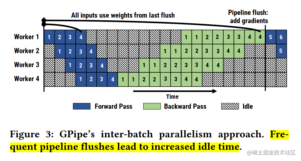
First, improve the parallelism of model training . On the basis of simple pipeline parallelism, Gpipe uses the idea of data parallelism to subdivide the mini-batch into multiple smaller micro-batches and send them to the GPU for training to improve the degree of parallelism.
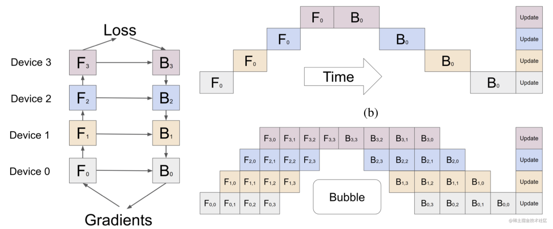
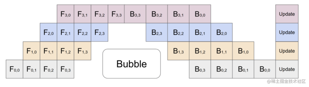
The above figure shows a comparison between simple pipeline parallelism and GPipe micro-batch pipeline parallelism. GPipe can effectively reduce the proportion of pipeline parallel bubble space. Among them, the first subscript of F represents the GPU number, and the second subscript of F represents the micro-batch number. Assume that we divide the mini-batch into M, then when the GPipe pipeline is parallelized, the Bubble time of the GPipe pipeline is: . Among them, K is the equipment, and M is how many micro-batches the mini-batch is divided into. When M>>K, this time can be ignored.
But this also has a disadvantage, that is, after splitting the batch into smaller sizes, the calculations for those layers that require statistics (such as Batch Normalization) will become cumbersome and need to be re-implemented. The method in Gpipe is to calculate and use the mean and variance in micro-batch during training, while continuously tracking the moving average and variance of all mini-batches for use in the testing phase. In this way, Layer Normalization is not affected.
Second, reduce video memory consumption through re-materialization . During forward propagation during model training, the calculation results of each operator are recorded and used for gradient calculation during back propagation.
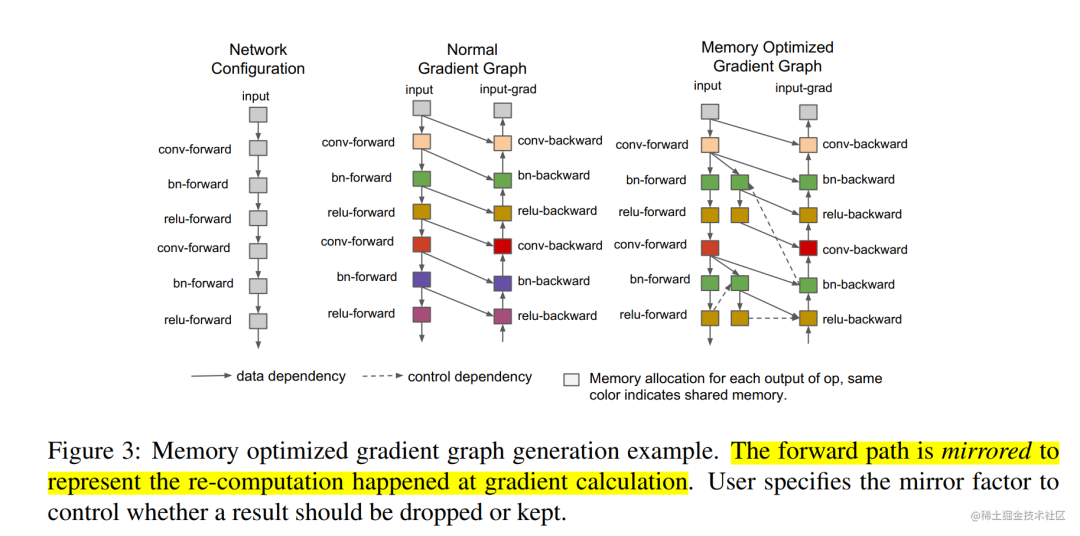
Re-materialization does not need to save the activation values output by the intermediate layer. When calculating the gradient, these activation values will be recalculated so that the gradient can be calculated. In GPipe, after applying this technology, if there are multiple layers on a device, then only the output value of the last layer among the multiple layers can be saved. This reduces the peak memory usage on each device, and the same model size requires less video memory.
Re-materialization does not mean that there is no need for intermediate results, but there is a way to calculate the intermediate results that were previously discarded in real time during the derivation process .
In short, GPipe solves the problem of being unable to train large models on a single device by dividing the model vertically; at the same time, it increases the degree of parallelism on multiple devices through micro-batch pipelines. In addition, it also uses re-materialization Reduced memory peak on a single device.
The GPipe pipeline parallel solution is described above. Next, we will talk about PipeDream. Before talking about PipeDream, let's first take a look at the pipeline parallel strategy.
Pipeline parallel strategy
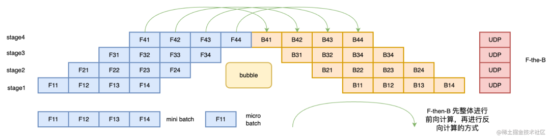
Pipeline parallelism can be divided into two modes: F-then-B and 1F1B according to the execution strategy. The simple pipeline parallelism and GPipe described before are both F-then-B models, while the PipeDream described later is a 1F1B model.
F-then-B strategy
F-then-B mode, forward calculation is performed first, and then reverse calculation is performed.
Because the F-then-B mode caches the intermediate variables and gradients of multiple micro-batches, the actual utilization of the video memory is not high.
1F1B Strategy
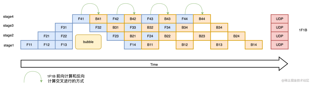
1F1B (One Forward pass followed by One Backward pass) mode is a way of interleaving forward calculation and reverse calculation. In 1F1B mode, forward calculation and reverse calculation are performed interleavedly, which can release unnecessary intermediate variables in time.
The 1F1B example is shown in the figure below, taking F42 of stage4 ( the forward calculation of the second micro-batch of stage4 ) as an example. Before F42 is calculated, the reverse B41 of F41 (the reverse calculation of the first micro-batch of stage4) Calculation) After the calculation is completed, the intermediate variables of F41 can be released, so that F42 can reuse the video memory of the intermediate variables of F41.
Research shows that compared with the F-then-B method, the 1F1B method can save 37.5% of the peak video memory. Compared with the simple pipeline parallel peak video memory, the peak video memory is significantly reduced, and the equipment resource utilization rate is significantly improved.
PipeDream (non-staggered 1F1B)-DeepSpeed
Gpipe's pipeline has the following problems:
After dividing the mini-batch into m micro-batch, it will cause more frequent pipeline refresh (Pipeline flush), which reduces the hardware efficiency and leads to an increase in idle time.
After the mini-batch is divided into m micro-batches, m activations need to be cached, which will lead to an increase in memory. The reason is that the intermediate result activation of each micro-batch forward calculation must be used by its backward calculation, so it needs to be cached in memory. Even if recalculation technology is used, the activation of forward calculation still needs to wait until the corresponding backward calculation is completed before it can be released.
The improvement method of PipeDream proposed by Microsoft DeepSpeed to address these problems is the 1F1B strategy. This improved strategy can solve the problem of cached activation copies, making the number of cached activations only related to the number of stages, thereby further saving video memory and training larger models. The solution is to strive to reduce the storage time of each activation, that is, each micro-batch data needs to complete the backward calculation as early as possible, so that each activation can be released as early as possible.
Note: Micro-batch is called micro-batch in GPipe and mini-batch in PipeDream . In order to avoid interference, this article uses micro-batch uniformly.
PipeDream’s specific solutions are as follows:
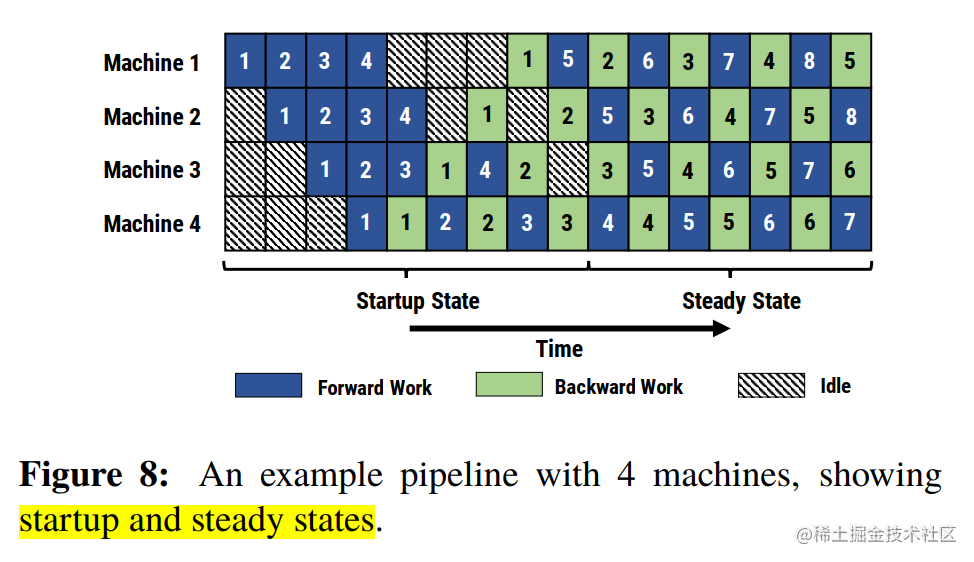
After a stage completes a micro-batch forward propagation, it immediately performs micro-batch backward propagation, and then releases resources, so that other stages can start calculation as early as possible. This is the 1F1B strategy . It's a bit like turning overall synchronization into asynchronous on many small data blocks, and many small data blocks are updated independently by everyone.
In the steady state of 1F1B, forward calculation/backward calculation will be strictly alternated on each machine, so that there will be a micro-batch data being processed on each GPU, thus ensuring resource utilization. High utilization (the entire pipeline is relatively balanced and there is no pipeline flush (Pipeline Flush), which ensures that parameter updates on each stage are executed at a fixed period.
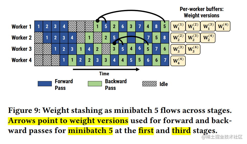
Faced with the asynchrony caused by the pipeline, 1F1B uses different versions of weights to ensure the effectiveness of training .
In addition, PipeDream has also extended 1F1B. For stages that use data parallelism, the round-robin scheduling mode is used to allocate tasks to various devices in the same stage, ensuring the forward propagation of a small batch of data. The calculation and backward propagation calculation occur on the same machine, which is 1F1B-RR (one-forward-noe-backward-round-robin).
Compared with GPipe, it seems that PipeDream has not optimized the Bubble rate. The PipeDrea pipeline Bubble time is still: . But after saving the video memory, if the device has a certain amount of video memory, you can reduce the Bubble rate by increasing the value of M (increasing the number of micro-batch).
PipeDream-2BW
The previous pipeline solutions GPipe and PipeDream had the following problems:
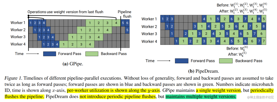
GPipe maintains a single version of the model weights, and the input mini-batches are divided into smaller micro-batches. Weight gradients are cumulative and not applied immediately, and the pipeline is refreshed periodically to ensure that multiple weight versions do not need to be maintained. GPipe provides weight update semantics similar to data parallelism, but periodic pipeline refreshes can be expensive, limiting throughput. One way to mitigate this overhead is to perform additional accumulations within the pipeline, but this is not always practical.
PipeDream uses a weight storage scheme to ensure that the same version of the weights is used in forward and backward passes of the same input. In the worst case, the total number of hidden weight versions is d, where d is the pipeline depth, which is too high for large models. Moreover, using PipeDream's default weight update semantics, the weight update of each stage (state) has different delay terms; at the same time, accumulation will not be performed in the pipeline.
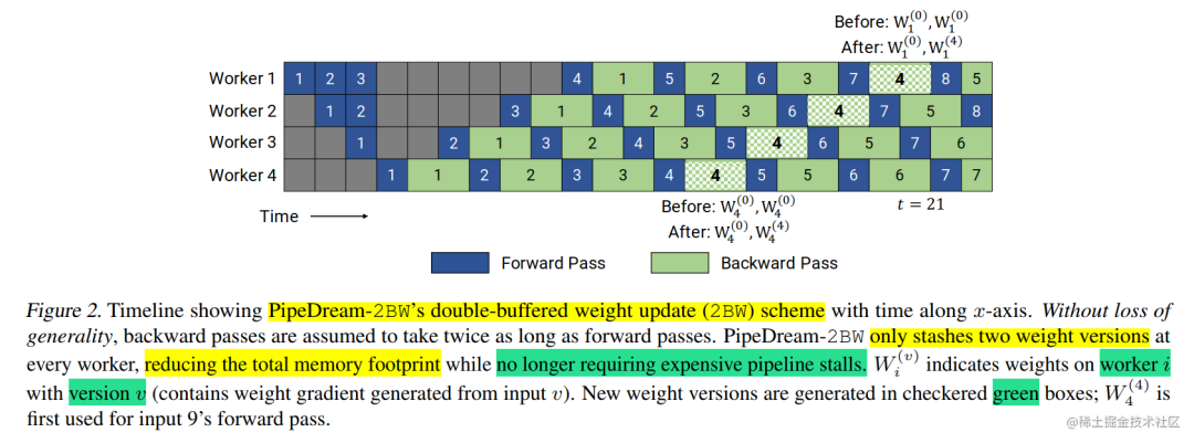
Based on this, the author proposed PipeDream-2BW. PipeDream-2BW only maintains two versions of model weights in the pipeline. 2BW is double-buffered weights.
PipeDream-2BW will generate a new weight version (m>=d) for every m micro-batches, where d is the pipeline depth, but because some remaining backward passes still depend on the old version of the model, the new model version Old versions cannot be replaced immediately, so the newly generated version of the weights needs to be buffered for future use. However, the total number of weight versions that need to be maintained is at most 2, because the weight versions used to generate new weight versions can be immediately discarded (subsequent inputs through this stage no longer use the old weight version), and since only two weight versions are saved version, which greatly reduces memory usage.
PipeDream-Flush(1F1B)
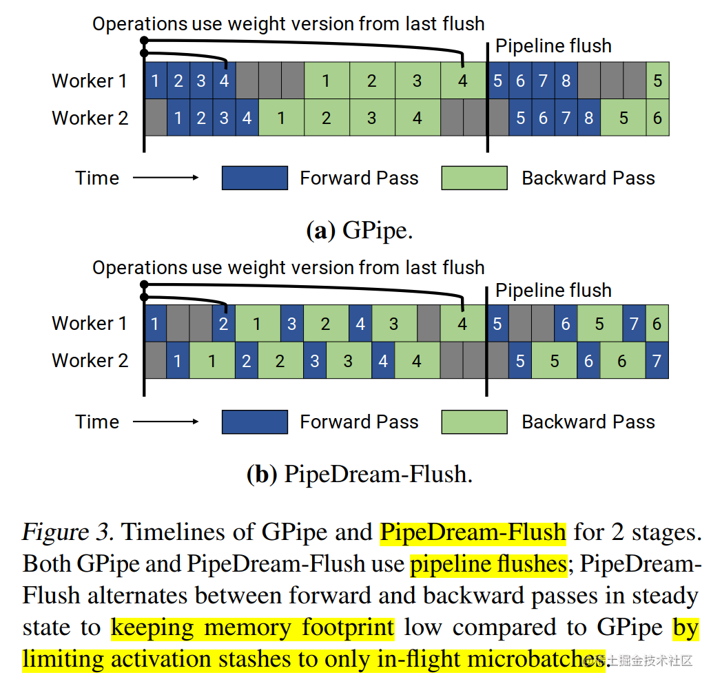
In the PipeDream 2BW paper (Memory-Efficient Pipeline-Parallel DNN Training), a variant PipeDream-Flush is also mentioned, using Flush to update weights. It has a lower memory footprint than PipeDream 2BW, but at the expense of lower throughput. This schedule reuses the 1F1B scheduling strategy in Microsoft's PipeDream; however, like GPipe, only a single weight version is maintained and regular pipeline flush is introduced to ensure that the weight version remains consistent during weight updates. In this way, Peak memory is reduced at the expense of execution performance. The figure below shows the timeline of PipeDream-Flush and GPipe with 2 pipeline stages.
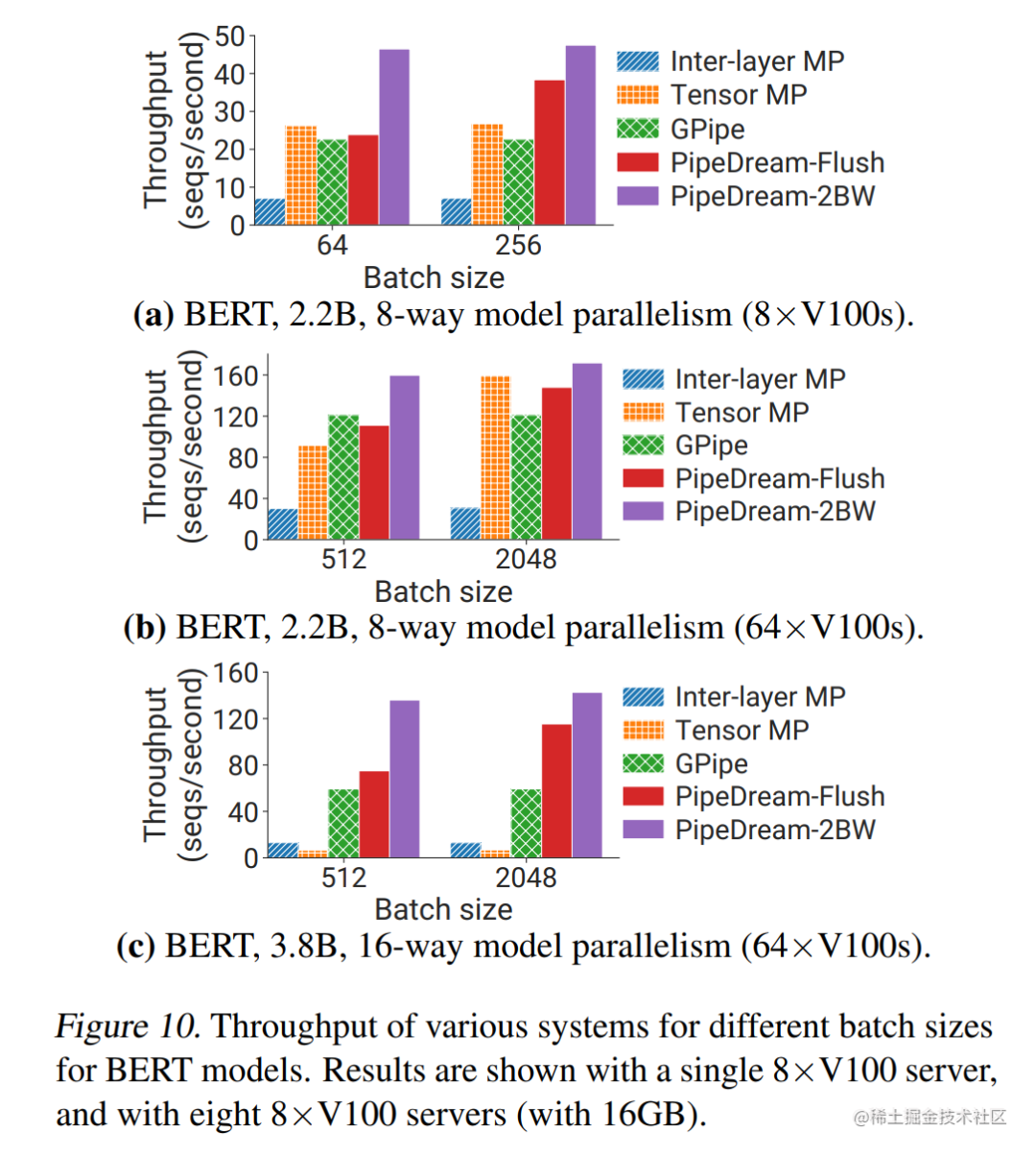
The figure below shows the throughput comparison of GPipe, PipeDream-Flush, and PipeDream 2BW pipeline parallel methods.
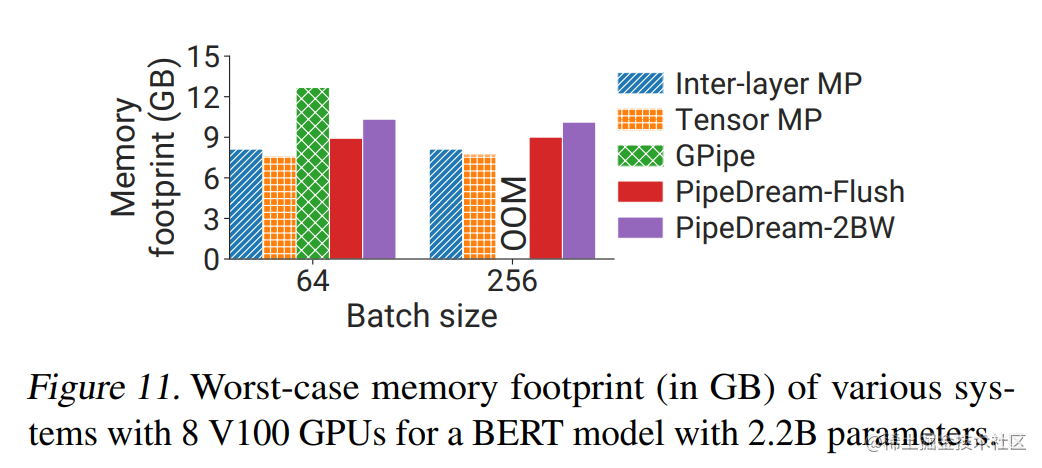
The figure below shows the memory comparison of GPipe, PipeDream-Flush, and PipeDream 2BW pipeline parallel methods.
1F1B schedule mode
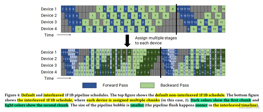
The above describes PipeDream. When using the 1F1B strategy, there are two scheduling modes: non-interleaved scheduling and interleaved scheduling. As shown in the figure below, the upper part shows the default non-interleaved schedule (non-interleaved schedule), and the bottom part shows the interleaved schedule (interleaved schedule).
non-interleaved scheduling
Non-interleaved scheduling can be divided into three phases. The first phase is a warm-up phase where the processor performs varying amounts of forward calculations. In the next phase, the processor performs a forward calculation and then a backward calculation. The last stage processor completes the backward calculation.
As mentioned above, Microsoft's PipeDream uses non-interleaved 1F1B scheduling. Although, this scheduling mode saves more memory than GPipe. However, it takes the same time as GPipe to complete a calculation round.
staggered scheduling
In interleaved scheduling, each device can perform computations on subsets of multiple layers (called model nuggets), rather than a collection of contiguous layers.
Specifically, in the previous non-staggered scheduling, device 1 has layers 1-4, device 2 has layers 5-8, and so on; but in interleaved scheduling, device 1 has layers 1, 2, 9, and 10 , device 2 has layers 3, 4, 11, 12, and so on. In the interleaved scheduling mode, each device on the pipeline is assigned to multiple pipeline stages (virtual stages), and each pipeline stage requires less calculation.
This mode saves both memory and time. But this scheduling mode requires that the number of micro-batch is an integral multiple of the pipeline stage (Stage).
Non-interleaved 1F1B scheduling is used in the paper related to NVIDIA Megatron-LM's pipeline parallelism (Efficient Large-Scale Language Model Training on GPU Clusters Using Megatron-LM).
PipeDream (Staggered 1F1B)-Megatron-LM
Megatron-LM proposed a small trick based on PipeDream-Flush: interleaved 1F1B scheduling, and interleaved 1F1B scheduling is also in the Megatron-LM paper (Efficient Large-Scale Language Model Training on GPU Clusters Using Megatron-LM), virtual pipeline) The most important innovation point.
Traditional pipeline parallelism usually places several consecutive model layers (such as Transformer layers) on a device. However, this paper on Megatron uses a virtual pipeline to perform interleaved 1F1B parallelism. When the number of devices remains unchanged, more pipeline stages are divided to increase the communication volume in exchange for a lower pipeline Bubble ratio.
For example, previously if each device had 4 layers (i.e. device 1 had layers 1 – 4, device 2 had layers 5 – 8, and so on), now we can have each device perform calculations on two model nuggets (each The model block has 2 layers), that is, device 1 has layers 1, 2, 9, and 10; device 2 has layers 3, 4, 11, and 12, and so on. With this scheme, each device in the pipeline is assigned multiple pipeline stages (each pipeline stage requires less computation than before).
Furthermore, this scheme requires that the number of microbatches in a mini-batch be an integral multiple of the pipeline parallelism size (the number of devices in the pipeline). For example, for 4 devices, the number of micro-batches in a mini-lot must be a multiple of 4.
So how does the virtual pipeline do it?
For example, if the network has 16 layers (numbered 0-15) and 4 Devices, the aforementioned Google's GPipe and Microsoft's PipeDream are divided into 4 stages, and Device1 and Layer 4-7 are placed according to the numbers 0-3. Put Device2, and so on.
Nvidia's virtual pipeline reduces the segmentation granularity according to the virtual_pipeline_stage concept proposed in the article. Taking virtaul_pipeline_stage=2 as an example, the 0-1 layer is placed on Device1, the 2-3 layer is placed on Device2,..., and the 6-7 layer is placed To Device4, layers 8-9 will continue to be placed on Device1, layers 10-11 will be placed on Device2,..., and layers 14-15 will be placed on Device4.
In this way, the number of point-to-point communications between Devices is directly doubled by virtual_pipeline_stage times, but the cavitation ratio is reduced. If it is defined that there are v virtual stages on each Device, or it is also called model chunks in the paper, in this In the example v=2, in this case, the cavitation ratio is:
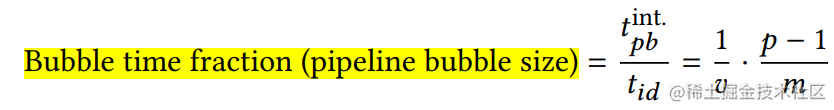
It can be seen from the above formula that the cavitation ratio is inversely proportional to v, which is reduced by v times. Of course, the reduction in pipeline bubble ratio is not without cost: this staggered scheduling requires additional communication. In terms of quantity, the communication volume has also increased by v times. Of course, we can reduce the impact of this additional communication by using high-speed network bandwidth in multi-GPU servers (eg DGX A100 nodes). The NVIDIA paper also discusses using eight InfiniBand network cards to reduce the impact of this additional communication.
Distributed training framework pipeline parallel solution
The above describes some of the current mainstream pipeline parallelism (PP) solutions. In general, PP can be subdivided into synchronous pipeline parallelism (Sync-PP) and asynchronous pipeline parallelism (Async-PP).
Representatives of Sync-PP include GPipe, PipeDream-flush, etc.;
Representatives of Async-PP include PipeDream, PipeDream-2BW, etc.
The synchronization method has the same weight update semantics as data parallelism, but requires the introduction of pipeline bubbles (idle waiting time), which will reduce training throughput. The asynchronous method completely eliminates bubbles in the training timeline, but different weight versions need to be introduced to solve the problem of weight expiration.
Let’s take a look at the pipeline parallelization schemes used in several well-known distributed training frameworks:
In PyTorch, the GPipe solution is used. The F-then-B scheduling strategy is used.
In DeepSpeed, PipeDream-Flush is used, using a non-interleaved 1F1B scheduling strategy. This scheduling scheme is used to facilitate the training of the largest models. During model training, storing multiple weight buffers can be prohibitive. Our primary goal is to have an "accurate" method without requiring convergence. trade off. Of course, the DeepSpeed engine component abstracts pipeline scheduling, and you can also implement other pipeline scheduling solutions by yourself.
In Megatron-LM, improvements are made based on PipeDream-Flush to provide a staggered 1F1B solution.
In Colossal-AI, the interleaved 1F1B scheme based on Megatron-LM provides non-interleaved (
PipelineSchedule) and interleaved (InterleavedPipelineSchedule) scheduling strategies.
Summarize
This article first describes simple pipeline parallelism, but simple pipeline parallelism is in a pipeline parallel group, and only one GPU is running at a time, which will result in extremely low GPU usage. Therefore, Google came up with Gpipe.
Gpipe uses the idea of data parallelism to subdivide the mini-batch into multiple smaller micro-batches and send them to the GPU for training to improve the degree of parallelism. After splitting the mini-batch into M micro-batches, it will lead to more frequent pipeline refreshes and reduce hardware efficiency. At the same time, after splitting into M micro-batches, each micro-batch will only use The previous activation value will, therefore, result in a larger memory footprint. Based on this, GPipe uses recalculation to solve the problem. The premise is that the recalculated result is the same as before, and the forward time cannot be too long, otherwise the pipeline will be stretched too much.
The two pipeline parallel strategies F-then-B and 1F1B are mentioned later. F-then-B may cause high memory usage. The PipeDream proposed by Microsoft solves the problem of excessive memory by reasonably arranging the order of forward and reverse processes (1F1B strategy).
Compared with GPipe, although PipeDream reduces memory usage, its bubble rate does not decrease. A non-interleaved 1F1B scheduling strategy is proposed in Megatron-LM's pipeline parallel solution. Further reduce the bubble rate. However, additional communication costs are incurred. Their paper mentions the use of IB networks to mitigate additional communication impacts.
As an aside, among the several pipeline parallel schemes described in this article, in addition to GPipe, Deepak Narayanan has participated in papers related to PipeDream and its variants, which is really productive.
If you think my article can help you, I look forward to your likes, collections and attention~~