1. Preview of algorithm operation renderings

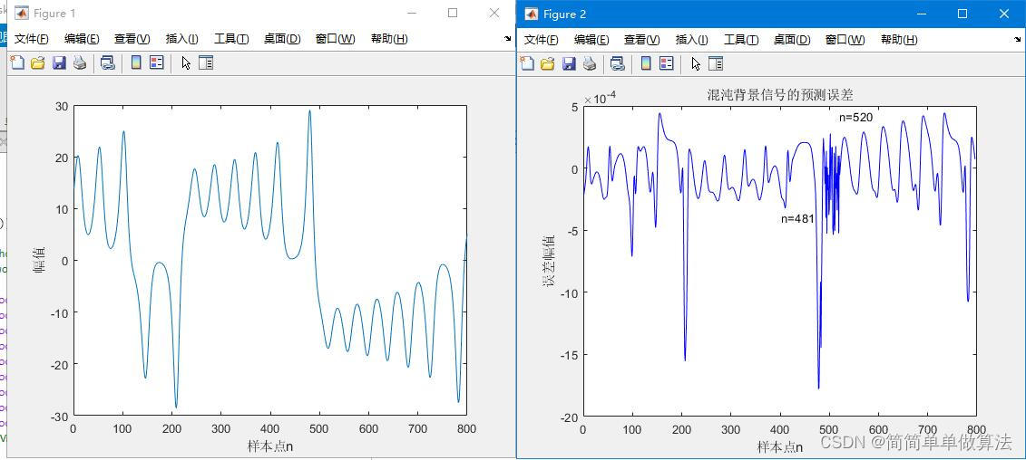
SVM:

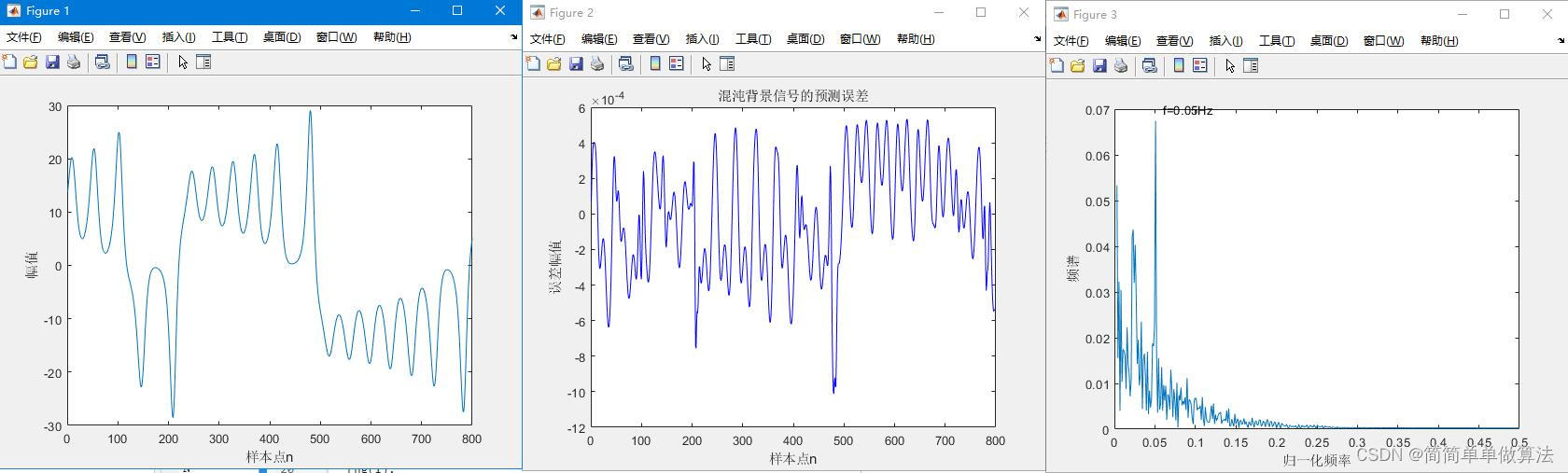
PSO-SVM:

GA-PSO-SVM:

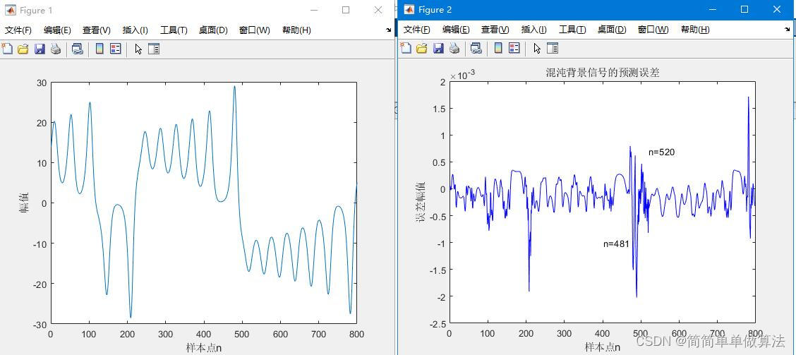
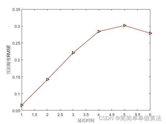
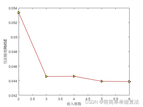
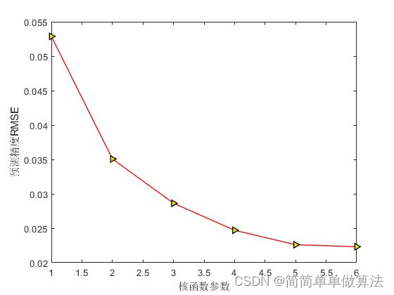
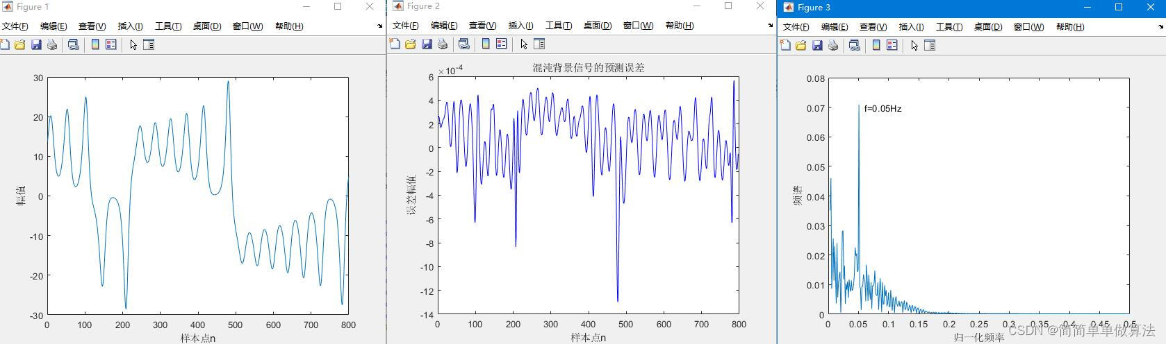The above simulation diagram refers to the literature "Research on Weak Signal Detection Method in Chaotic Background Based on Phase Space Reconstruction"

2.Algorithm running software version

MATLAB2022a

3. Some core programs

................................................
while gen < MAXGEN;   
      gen
      w       = wmax-gen*(wmax-wmin)/MAXGEN;
      FitnV = ranking(Objv);    
      Selch = select('sus',Chrom,FitnV);    
      Selch = recombin('xovsp',Selch,0.9);   
      Selch = mut(Selch,0.1);   
      phen1 = bs2rv(Selch,FieldD);   
      %基于粒子群的速度更新
      for i=1:1:NIND
          if gen > 1
              va(i)  = w*va(i) + c1*rand(1)*(phen1(i,1)-taos2)   + c2*rand(1)*(taos-taos2);
              vb(i)  = w*vb(i) + c1*rand(1)*(phen1(i,2)-ms2)     + c2*rand(1)*(ms-ms2);
              vc(i)  = w*vc(i) + c1*rand(1)*(phen1(i,3)-Cs2)     + c2*rand(1)*(Cs-Cs2);
              vd(i)  = w*vd(i) + c1*rand(1)*(phen1(i,4)-gammas2) + c2*rand(1)*(gammas-gammas2);
          else
              va(i)  = 0;
              vb(i)  = 0;
              vc(i)  = 0;
              vd(i)  = 0;
          end
      end
      
      for a=1:1:NIND  
          Data1(a,:) = phen1(a,:);      
          tao        = round(Data1(a,1) + 0.15*va(i));%遗传+PSO
          m          = round(Data1(a,2) + 0.15*vb(i));
          C          = Data1(a,3)       + 0.15*vc(i);
          gamma      = Data1(a,4)       + 0.15*vd(i);
          
            if tao >= max1
               tao  = max1;
            end
            if tao <= min1
               tao  = min1;
            end     
            if m >= max2
               m = max2;
            end
            if m <= min2
               m = min2;
            end  
            if C >= max3
               C = max3;
            end
            if C <= min3
               C = min3;
            end  
            if gamma >= max4
               gamma = max4;
            end
            if gamma <= min4
               gamma = min4;
            end   

            
          %计算对应的目标值
          [epls,tao,m,C,gamma] = func_fitness(X_train,X_test,tao,m,C,gamma);
          E                    = epls;
          JJ(a,1)              = E;
      end 
      
      Objvsel=(JJ);    
      [Chrom,Objv]=reins(Chrom,Selch,1,1,Objv,Objvsel);   
      gen=gen+1; 

      %保存参数收敛过程和误差收敛过程以及函数值拟合结论
      Error(gen) = mean(JJ);
      pause(0.2);
      [V,I] = min(Objvsel);
      JI      = I;
      tmpps    = Data1(JI,:);
      taos2    = round(tmpps(1));
      ms2      = round(tmpps(2));
      Cs2      = tmpps(3);
      gammas2  = tmpps(4);
end 
 
[V,I] = min(Objvsel);
JI      = I;
tmpps   = Data1(JI,:);
tao0    = round(tmpps(1));
m0      = round(tmpps(2));
C0      = tmpps(3);
gamma0  = tmpps(4);

  
%save GAPSO.mat tao0 m0 C0 gamma0
end




if SEL == 2
load GAPSO.mat
%调用四个最优的参数
tao   = tao0;
m     = m0;
C     = C0;
gamma = gamma0;



%先进行相空间重构
[Xn ,dn ] = func_CC(X_train,tao,m);
[Xn1,dn1] = func_CC(X_test,tao,m);

t  = 1/1:1/1:length(dn1)/1;
f  = 0.05;
sn = 0.0002*sin(2*pi*f*t);
%叠加
dn1 = dn1 + sn';
 
%SVM训练%做单步预测
cmd = ['-s 3',' -t 2',[' -c ', num2str(C)],[' -g ',num2str(gamma)],' -p 0.000001']; 
model = svmtrain(dn,Xn,cmd);
%SVM预测
[Predict1,error1] = svmpredict(dn1,Xn1,model);
RMSE              = sqrt(sum((dn1-Predict1).^2)/length(Predict1));
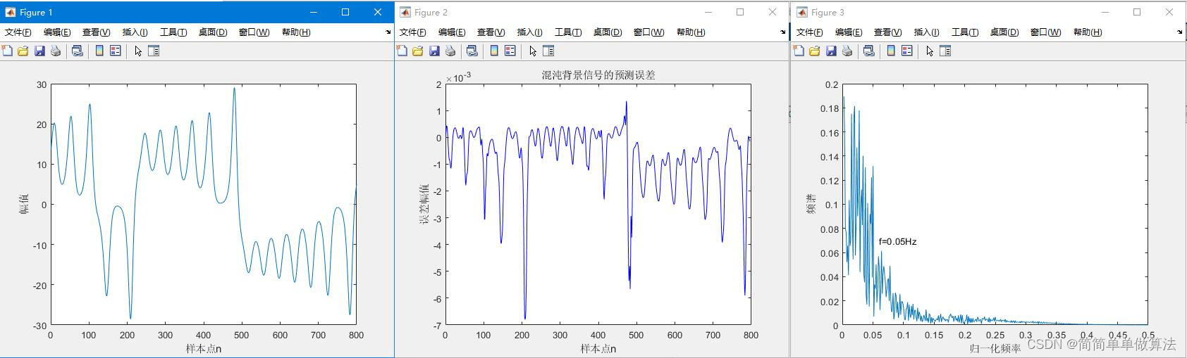
Err               = dn1-Predict1;
%误差获取
clc;
RMSE 
 





figure;
plot(Err,'b');
title('混沌背景信号的预测误差'); 
xlabel('样本点n');
ylabel('误差幅值');

Fs = 1;
y  = fftshift(abs(fft(Err)));
N  = length(y)
fc = [-N/2+1:N/2]/N*Fs;

figure;
plot(fc(N/2+2:N),y(N/2+2:N));
xlabel('归一化频率');
ylabel('频谱');
text(0.06,0.07,'f=0.05Hz');

end
07_006m

4. Overview of algorithm theory

4.1 SVM

Support Vector Machine (SVM) is a machine learning method for classification and regression. Its principle is based on finding an optimal hyperplane (or curve in non-linear cases) to divide different categories of data points. The goal of SVM is to find a hyperplane that maximizes the margin between different categories, thereby achieving good generalization ability on unknown data.

The goal of SVM is to find a hyperplane that maximizes the distance (margin) from the nearest data point (support vector) to the hyperplane. This interval can be expressed as the functional distance from the data point to the hyperplane, that is:

The goal of SVM is to solve the following optimization problem:

In nonlinear situations, SVM can map data from the original feature space to a high-dimensional feature space by introducing a kernel function to find a hyperplane in the high-dimensional space for classification. Common kernel functions include linear kernel, polynomial kernel, Gaussian kernel (RBF kernel), etc.
To sum up, the principle of SVM is to find an optimal hyperplane or curve that maximizes the distance between different categories to achieve the classification task. Its advantage lies in its ability to handle high-dimensional data, nonlinear problems, and its ability to resist overfitting to a certain extent.

4.2 PSO-SVM

In the optimization process of applying PSO to SVM, we mainly focus on the hyperparameters of SVM, such as kernel function type, regularization parameter C, etc. The PSO algorithm can help us find a set of hyperparameters that make SVM perform best on the training data.

In PSO-SVM, the fitness function is usually the performance index of SVM on the training set, such as accuracy rate, F1 score, etc. Optimizing the hyperparameters of SVM through the PSO algorithm can help us find an optimal set of hyperparameter configurations, thereby improving the performance of SVM in classification problems. This method can automatically search the hyperparameter space to a certain extent, avoiding the tedious process of manual adjustment.

4.3 GA-PSO-SVM

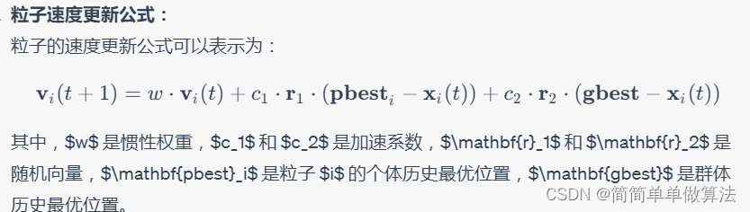
GA-PSO combines the population evolution of genetic algorithms and the local search capabilities of particle swarm optimization. Genetic algorithms simulate the process of biological evolution and optimize individuals in the population through operations such as crossover and mutation. Particle swarm optimization simulates the behavior of groups in nature such as flocks of birds or fish, and adjusts the position of particles through individual historical optimality and group historical optimality.

In the optimization process of applying GA-PSO to SVM, we mainly focus on the hyperparameters of SVM, such as kernel function type, regularization parameter C, etc. The GA-PSO algorithm can help us search for better solutions in the hyperparameter space to improve the performance of SVM on training data. The formulas of GA-PSO include the selection, crossover and mutation operations of genetic algorithms, as well as the speed and position update formulas of particle swarm optimization. These formulas can be adapted to specific algorithm variants.

In general, the GA-PSO algorithm combines genetic algorithm and particle swarm optimization, and realizes the optimization of SVM hyperparameters through the global search of genetic algorithm and the local search of particle swarm optimization, as well as the performance evaluation of SVM. This approach allows for a more comprehensive search of the hyperparameter space, which improves the performance of SVMs in classification problems.

5. Algorithm complete program engineering

OOOOO

OOO

Matlab simulation of weak signal detection algorithm in chaotic background based on phase space reconstruction, comparing SVM, PSO-SVM and GA-PSO-SVM