1. Software version
matlab2013b
2. Theoretical knowledge of this algorithm
The problem is, suppose I have a collection track with 5 collection piles on it, these 5 collection piles are regarded as a 4*20 matrix (only 4*10 below), each module (for example: A31 and A32's different element content), in order to meet the requirements of the number of collected items and element content (for example: 5 tons to be collected and a unit mass of an element between 65 and 62), find out which module is taken in each 4*20 matrix out to meet the requirements and find the most optimal track?


Known data:
1. The element content of each collection pile (in sheet 1 of the excel table)
2. The coordinates of the modules in each collection stack, the length, width and height (in meters) (in sheet 1 of the excel sheet)
3. Requirements for element content and the number of collected items (in sheet 2 of the excel form), there are five maximum and minimum values for different contents, as well as the requirements for the number of collected items, as well as errors.
4. The two collection piles on the left side of the track are of type C and type A respectively, and the distance between the two collection piles is 30m; the three collection piles on the right side of the track are B type, B type and C type in order. Likewise, the distance between each collection stack is 20m. 5. Collection heap shapes are attached in Appendix 1
Appendix 1 Acquisition of Contralateral Views
Height: 10m (A.BC)
The width and length of each layer are different, the specific data is in the excel table
So the first row is the volume of the triangle, and the rest are the volume of the ladder row.

This is actually an optimization problem, that is, to meet the needs of collecting items, it is necessary to load 5 distribution centers of 3 types, and only the top one can be taken each time. If the item at the current position is not taken at least , then you can only take the top item first, then count the distance of the loading trajectory, and calculate the shortest distance through optimization.
Then, the key to solving the problem here is to calculate the objective function, and then use the optimization algorithm to optimize the objective function. The main goal of this algorithm is the design of the objective function, which is also the difficulty of the subject.
First, according to the above requirements, we establish the following mathematical model:
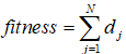
Here, dj represents the distance from one module to another each time. If it is moved from one collection pile to another collection pile, then the distance between the collected modules is calculated in the other pile.
So the above formula is:
That is, the sum of all distances at different acquisition stacks. Here, two factors need to be considered through optimization, the movement between the different acquisition stacks, and how the acquisition of the module is performed on each acquisition.
Our goal is to minimize the value of the above function, so as to obtain the collection route trajectory.
Here, the difficulties that need to be considered are as follows:
First: the spatial trajectory is three-dimensional, which is more complicated than two-dimensional.
Second: the establishment of constraints, we establish the following constraints according to the needs of the project.
2.1 Collection rule constraints.
That is, only the top one can be collected each time. If the top one is not taken away, the bottom one cannot be directly collected.
Here, we use the mathematical formula as follows:

Mark the modules of the four layers respectively. The top one is 4. If it is taken away, it will be directly assigned 0. In this way, we can only go to the one with the largest label each time. If it is taken away, then the value that was taken is 0, then when judging, you can take the following, if all are taken away, it is all 0, if it is all zero, then this column cannot take a value . That is, all zeros are empty.
2.2 Satisfy the constraints on the number of collected items and element content
According to the data provided, the maximum number of items is 60000t with an error of 1.
The element content is the constraint condition:
| element 1 |
element 2 |
element 3 |
element 4 |
element 5 |
|
| 65 |
6 |
4 |
0.077 |
0.1 |
maximum value |
| 62 |
0 |
0 |
0 |
0 |
minimum |
According to the constraints given by the subject, we need to pass the acquisition module to make the final total weight 60000, and the influence of the proportion of each element in the collected items satisfies the above constraints.
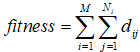
That is to say, the above constraint condition is to collect the items so that the total amount meets the requirements, and the unit mass of the five elements satisfies the above constraints, and finally the collection trajectory is the shortest.
Therefore, through the above comprehensive analysis, the mathematical formula we want is:

For convenience, we organize the required data in excel, and convert some of the data you edited with formulas into real data. The modified excel file can be seen in the newly sent data, and the constraints are set directly in the program.
Here, we assume that when the device moves from one endpoint to another, it gradually moves forward, not back and forth. That is, the device is moved from one end of the track to the other at a time (in fact, the rules are to move in sequence)
According to this assumption, the idea of our design is that when moving to a pile, first collect on this pile of items, because the distance between each pile of items is much larger than the distance between each module inside each pile, So in practice, it is impossible to switch the grab module back and forth between two different heaps, which is also in line with our assumption above.
According to the above assumption, the order we grab is B heap, C heap, A heap, A heap, B heap.
3. Core code
%根据这个假设,我们设计的思路为当每次运动到一堆的时候,首先在这一堆物品上进行采集,由于
%每堆物品之间的间距远大于每堆内部的各个模块之间的间隔,所以在实际中也不可能在两个不同的
%堆之间来回切换的抓取模块,这也符合我们上面的假设。
%根据上面的假设,我们抓取的顺序为B堆,C堆,A堆,A堆,B堆。
%这里,我们所使用的算法是局部PSO优化,然后再整体PSO优化的算法,即首先通过再每一堆的采集
%的时候进行PSO优化,并使的各个元素含量满足约束的条件下,得到路径最短的采集轨迹,然后通过
%后面三堆重复相同的优化算法,最后第五堆的时候,在做相同的优化前提下,同时检测总量是否满足
%条件,如果不满足进入下一次大迭代循环,然后重复上面的操作,最后得到满足条件的总的采集轨迹。

clc;
clear;
close all;
warning off;
pack;
addpath 'func\'

%**********************************************************************************
%步骤一:调用数据
%步骤一:调用数据
Dat = xlsread('Dat\datas.xlsx');

%分成ABC三组
A_set = Dat( 1:40 ,:);
B_set = Dat(41:80 ,:);
C_set = Dat(81:120,:);


%A相关数据
%坐标
A_POS = A_set(:,1:3);
%元素含量
A_FAC = A_set(:,4:8);
%体积长宽高
A_VUM = A_set(:,9:11);


%B相关数据
%坐标
B_POS = B_set(:,1:3);
%元素含量
B_FAC = B_set(:,4:8);
%体积长宽高
B_VUM = B_set(:,9:11);


%C相关数据
%坐标
C_POS = C_set(:,1:3);
%元素含量
C_FAC = C_set(:,4:8);
%体积长宽高
C_VUM = C_set(:,9:11);


%**************************************************************************
%**************************************************************************

%**********************************************************************************
%步骤二:参数初始化
%步骤二:参数初始化
%约束参数
%59999 ~ 60001
Mass_all = 60000;
Mass_err = 1;
%元素1
Mass1_max= 65;
Mass1_min= 62;
%元素2
Mass2_max= 6;
Mass2_min= 0;
%元素3
Mass3_max= 4;
Mass3_min= 0;
%元素4
Mass4_max= 0.077;
Mass4_min= 0;
%元素5
Mass5_max= 0.1;
Mass5_min= 0;

%优化算法参数
%优化算法参数
%迭代次数
Iteration_all = 1;
Iteration_sub = 10000;
%粒子数目
Num_x     = 200;

%密度
P         = 2.1;
%计算各个模块的质量,单位t
%注意,本课题一个堆中有个四个形状的模块,即三角形,三种梯形,所以我们根据长宽高以及对应的形状计算体积,从而计算质量
A_Vulome = func_cal_volume(A_VUM);
B_Vulome = func_cal_volume(B_VUM);
C_Vulome = func_cal_volume(C_VUM);
%计算每个采集堆的各个模块的质量
A_mass   = P*A_Vulome;
B_mass   = P*B_Vulome;
C_mass   = P*C_Vulome;

%以下根据实际轨迹上的堆的分布来设置
maxs_sets = [B_mass;C_mass;A_mass;A_mass;B_mass];
FAC_sets  = [B_FAC;C_FAC;A_FAC;A_FAC;B_FAC];


%**************************************************************************
%**************************************************************************

%**********************************************************************************
%步骤三:开始优化运算
%步骤三:开始优化运算
X_pos{1} = B_POS(:,1);
Y_pos{1} = B_POS(:,2);
Z_pos{1} = B_POS(:,3);

X_pos{2} = C_POS(:,1);
Y_pos{2} = C_POS(:,2);
Z_pos{2} = C_POS(:,3);

X_pos{3} = A_POS(:,1);
Y_pos{3} = A_POS(:,2);
Z_pos{3} = A_POS(:,3);

X_pos{4} = A_POS(:,1);
Y_pos{4} = A_POS(:,2);
Z_pos{4} = A_POS(:,3);

X_pos{5} = B_POS(:,1);
Y_pos{5} = B_POS(:,2);
Z_pos{5} = B_POS(:,3);


%先通过PSO优化需求模型
for Num_pso = 4:40%这里没有必要设置太大,设置大了需求量肯定会超过60000,因此,这个值得大小根据需求量来确定,大概范围即可
    Num_pso
    x = zeros(Num_x,Num_pso);

    i = 0;

    %产生能够满足采集规则的随机粒子数据
    for jj = 1:Num_x
        %产生随机数的时候,必须是先采集第一层,然后才采集第二层,依次类推
        %第1层
        index1 = [1:10,41:50,81:90,121:130,161:170];
        %第2层
        index2 = [1:10,41:50,81:90,121:130,161:170]+10;
        %第3层
        index3 = [1:10,41:50,81:90,121:130,161:170]+20;
        %第4层
        index4 = [1:10,41:50,81:90,121:130,161:170]+30;

        %根据采集规则产生随机数
        %根据采集规则产生随机数
        %根据采集规则产生随机数
        index  = [index1;index2;index3;index4];

        i = 0;
        while i < Num_pso
            i = i + 1;
            if i> 1
                for j = 1:50;
                    index(IS(j),ind(1)) = 9999;
                end
            end

            for j = 1:50;
                [VS,IS(j)] = min(index(:,j));
                tmps(1,j)  = index(IS(j),j);
            end
            ind  = randperm(40);
            a(i) = tmps(ind(1));
            if a(i) == 9999
               i = i-1;
            end
        end

        x(jj,:) = a;

    end


    n             = Num_pso;
    F             = fitness_mass(x,maxs_sets,Mass_all);
    Fitness_tmps1 = F(1);
    Fitness_tmps2 = 1;

    for i=1:Num_x
        if Fitness_tmps1 >= F(i)
           Fitness_tmps1 =  F(i);
           Fitness_tmps2 =  i;
        end
    end
    xuhao      = Fitness_tmps2;
    Tour_pbest = x;                        %当前个体最优
    Tour_gbest = x(xuhao,:) ;              %当前全局最优路径
    Pb         = inf*ones(1,Num_x);        %个体最优记录
    Gb         = F(Fitness_tmps2);         %群体最优记录
    xnew1      = x;
    N          = 1;

    while N <= Iteration_sub
        %计算适应度
        F = fitness_mass(x,maxs_sets,Mass_all);
        for i=1:Num_x
            if F(i)<Pb(i)
               %将当前值赋给新的最佳值
               Pb(i)=F(i);
               Tour_pbest(i,:)=x(i,:);
            end

            if F(i)<Gb
               Gb=F(i);
               Tour_gbest=x(i,:);
            end
        end

        Fitness_tmps1 = Pb(1);
        Fitness_tmps2 = 1;

        for i=1:Num_x
            if Fitness_tmps1>=Pb(i)
               Fitness_tmps1=Pb(i);
               Fitness_tmps2=i;
            end
        end

        nummin = Fitness_tmps2;
        %当前群体最优需求量差
        Gb(N)  = Pb(nummin);

        for i=1:Num_x
            %与个体最优进行交叉
            c1 = round(rand*(n-2))+1;
            c2 = round(rand*(n-2))+1;
            while c1==c2
                  c1 = round(rand*(n-2))+1;
                  c2 = round(rand*(n-2))+1;
            end
            chb1 = min(c1,c2);
            chb2 = max(c1,c2);
            cros = Tour_pbest(i,chb1:chb2);
            %交叉区域元素个数
            ncros= size(cros,2);
            %删除与交叉区域相同元素
            for j=1:ncros
                for k=1:n
                    if xnew1(i,k)==cros(j)
                       xnew1(i,k)=0;
                       for t=1:n-k
                           temp=xnew1(i,k+t-1);
                           xnew1(i,k+t-1)=xnew1(i,k+t);
                           xnew1(i,k+t)=temp;
                       end
                    end
                end
            end
            xnew = xnew1;
            %插入交叉区域
            for j=1:ncros
                xnew1(i,n-ncros+j) = cros(j);
            end
            %判断产生需求量差是否变小
            masses=0;
            masses = sum(maxs_sets(xnew1(i,:)));
            if F(i)>masses
               x(i,:) = xnew1(i,:);
            end

            %与全体最优进行交叉
            c1 = round(rand*(n-2))+1;
            c2 = round(rand*(n-2))+1;
            while c1==c2
                  c1=round(rand*(n-2))+1;
                  c2=round(rand*(n-2))+1;
            end
            chb1 = min(c1,c2);
            chb2 = max(c1,c2);
            %交叉区域矩阵
            cros = Tour_gbest(chb1:chb2);
            %交叉区域元素个数
            ncros= size(cros,2);
            %删除与交叉区域相同元素
            for j=1:ncros
                for k=1:n
                    if xnew1(i,k)==cros(j)
                       xnew1(i,k)=0;
                       for t=1:n-k
                           temp=xnew1(i,k+t-1);
                           xnew1(i,k+t-1)=xnew1(i,k+t);
                           xnew1(i,k+t)=temp;
                       end
                    end
                end
            end
            xnew = xnew1;
            %插入交叉区域
            for j=1:ncros
                xnew1(i,n-ncros+j) = cros(j);
            end
            %判断产生需求量差是否变小
            masses=0;
            masses = sum(maxs_sets(xnew1(i,:)));
            if F(i)>masses
              x(i,:)=xnew1(i,:);
            end
            %进行变异操作
            c1          = round(rand*(n-1))+1;
            c2          = round(rand*(n-1))+1;
            temp        = xnew1(i,c1);
            xnew1(i,c1) = xnew1(i,c2);
            xnew1(i,c2) = temp;
            %判断产生需求量差是否变小
            masses=0;
            masses = sum(maxs_sets(xnew1(i,:)));

            if F(i)>masses
               x(i,:)=xnew1(i,:);
            end
        end

        Fitness_tmps1=F(1);
        Fitness_tmps2=1;
        for i=1:Num_x
           if Fitness_tmps1>=F(i)
              Fitness_tmps1=F(i);
              Fitness_tmps2=i;
           end
        end
        xuhao      = Fitness_tmps2;
        L_best(N)  = min(F);
        %当前全局最优需求量
        Tour_gbest = x(xuhao,:);
        N          = N + 1;

    end
    %判断含量是否满足要求
    for ii = 1:5
        Fac_tmps(ii) = sum(FAC_sets(Tour_gbest,ii)'.*maxs_sets(Tour_gbest))/sum(maxs_sets(Tour_gbest));
    end

    if (Fac_tmps(1) >= Mass1_min & Fac_tmps(1) <= Mass1_max) &...
       (Fac_tmps(2) >= Mass2_min & Fac_tmps(2) <= Mass2_max) &...
       (Fac_tmps(3) >= Mass3_min & Fac_tmps(3) <= Mass3_max) &...
       (Fac_tmps(4) >= Mass4_min & Fac_tmps(4) <= Mass4_max) &...
       (Fac_tmps(5) >= Mass5_min & Fac_tmps(5) <= Mass5_max)
       flag(Num_pso-3) = 1;
    else
       flag(Num_pso-3) = 0;
    end
    Mass_fig(Num_pso-3)  = min(L_best);
    Mass_Index{Num_pso-3}= Tour_gbest ;
end

figure;
plot(Mass_fig,'b-o');
xlabel('采集模块个数');
ylabel('需求量计算值和标准需求量的差值关系图');

save temp\result1.mat Mass_fig Mass_Index flag
4. Operation steps and simulation conclusion
First, run the program run_first.m to search all acquisition methods for acquisition combinations with a demand between 59999 and 60001. and save the simulation results.
The simulation results of this step are as follows:

Through this step, a module set that meets the acquisition rules and element content and meets the demand will be optimized, and then run_second.m will be run to optimize the trajectory.
The final optimized demerit is obtained, that is, the shortest trajectory length under the conditions

5. References
A06-10
6. How to obtain the complete source code
Method 1: Contact the blogger via WeChat or QQ
Method 2: Subscribe to the MATLAB/FPGA tutorial, get the tutorial case and any 2 complete source code for free