Transformer-based text sentiment analysis (Keras version)

I. Introduction

Since 2017, the RNN series of networks has been gradually replaced by a network called Transformer. Now Transformer has become the mainstream model in natural language processing, and Transformer has led to a big boom in language models. From Bert to GPT3, and now to ChatGPT. Transformer has achieved functions unimaginable by humans and is still developing.

This article will implement text sentiment analysis tasks based on the Encoder part of Transformer.

2. Data processing

For data processing, you can refer to the code of the previous text sentiment analysis based on LSTM (Keras version) . This article uses another simple method to implement it.

2.1 Data Preview

First, you need to download the corresponding data: ai.stanford.edu/~amaas/data… . Click on the location in the picture below:

After the data is decompressed, the following directory structure is obtained:
After the data is decompressed, the following directory structure is obtained:

- aclImdb
    - test
        - neg
        - pos
        - labeledBow.feat
        - urls_neg.txt
        - urls_pos.txt
    - train
        - neg
        - pos

This is a movie review data set. The reviews contained in neg are reviews with lower ratings, while the reviews contained in pos are reviews with higher ratings. The data we need are neg and pos in test, and neg and pos in train (neg means negative, pos means positive). Let's start processing it below.

2.2 Import module

Before starting to write code, you need to import the relevant modules:

import os
import keras
import tensorflow as tf
from keras import layers

My environment is tensorflow2.7. Some versions of tensorflow have different import methods. You can replace them according to your own environment.

2.3 Read data

Define a function here to read the comment file:

def load_data(data_dir=r'/home/zack/Files/datasets/aclImdb/train'):
    """
    data_dir：train的目录或test的目录
    输出：
        X：评论的字符串列表
        y：标签列表（0,1）
    """
    classes = ['pos', 'neg']
    X, y = [], []
    for idx, cls in enumerate(classes):
        # 拼接某个类别的目录
        cls_path = os.path.join(data_dir, cls)
        for file in os.listdir(cls_path):
            # 拼接单个文件的目录
            file_path = os.path.join(cls_path, file)
            with open(file_path, encoding='utf-8') as f:
                X.append(f.read().strip())
                y.append(idx)
    return X, np.array(y)

The above function will get two lists for us to process later.

2.4 Build vocabulary and tokenize

The processing of the previous part is the same as the previous article, and the operation of constructing vocabulary and tokenize is implemented by keras api. code show as below:

X, y = load_data()
vectorization = TextVectorization(max_tokens=vocab_size, output_sequence_length=seq_len)
# 构建词表
vectorization.adapt(X)
# tokenize
X = vectorization(X)

The adapt method receives a sentence list. After calling the adapt method, keras will help us build a word list, and then use vectorization (X) to convert the sentence list into a word id list.

3. Build a model

The Encoder part of Transformer is used here as the backbone of our network. We need to implement two parts, namely PositionalEmbedding and TransformerEncoder, and form the two parts into an emotion classification model.

3.1 TransformerEncoder

Let’s briefly introduce Transformer. Here’s a rough look at the various components of Transformer. The Transformer structure is as follows:

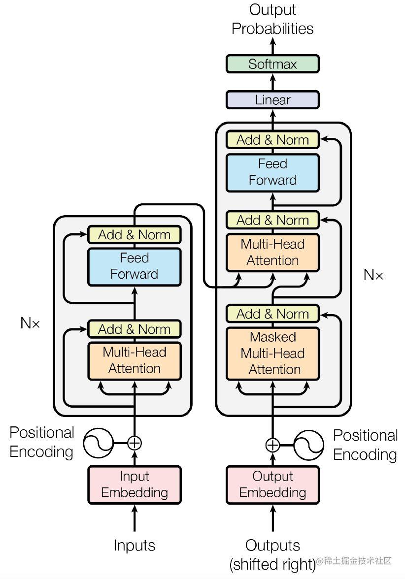
The left half is the Encoder and the right half is the Decoder. What we want to implement is the Encoder part. Let's take a look at the Decoder part from the bottom up.

（1）Input Embedding和Positional Encoding

The input of the Transformer is a list of ids with a shape of batch_size × sequence_len. The input will first go through a simple Embedding layer (Input Embedding) to obtain a shape of batch_size × sequence_len × embed_dim, which we call te. teIt contains sequence_lenword embeddings, tethe first embedding of which will pe[0]be added to the vector, tethe second embedding of will t[1]be added to the vector, and so on.

Therefore pe, the shape should be sequence_len × embed_dim, pewhich contains the position information. In the original paper, pethere is a fixed formula to obtain, and the position information is fixed peafter . However, this paper replaces it with a method called Positional Embedding during implementation. The implementation code is as follows:

class PositionalEmbedding(layers.Layer):
    def __init__(self, input_size, seq_len, embed_dim):
        super(PositionalEmbedding, self).__init__()
        self.seq_len = seq_len
        # 词嵌入
        self.tokens_embedding = layers.Embedding(input_size, embed_dim)
        # 位置嵌入
        self.positions_embedding = layers.Embedding(seq_len, embed_dim)

    def call(self, inputs, *args, **kwargs):
        # 生成位置id
        positions = tf.range(0, self.seq_len, dtype='int32')
        te = self.tokens_embedding(inputs)
        pe = self.positions_embedding(positions)
        return te + pe

An idea similar to word embedding is used here, allowing the network to learn location information by itself.

（2）Multi-Head Attention

Multi-Head Attention can be thought of as doing multiple Self-Attentions on a sequence, and then splicing the structures of each Self-Attention together. There are corresponding implementations in Keras and Pytorch. Here we look at how to use them.

When creating the MultiHeadAttention layer, you need to specify the number of heads and the dimension of the key. During forward propagation, if two identical sequences are passed in, Self-Attention is being done. The code is as follows:

from keras import layers
import tensorflow as tf

# 形状为batch_size × sequence_len × embed_dim
X = tf.random.uniform((3, 10, 5))
mta = layers.MultiHeadAttention(4, 10)
out = mta(X, X)
# 输出：(3, 10, 5)
print(out.shape)

It can be seen from the code that the input and output shapes of MultiHeadAttention are consistent.

（3）Add & Norm

After Attention, we put the Attention input and Attention output into a module called Add & Norm. Here we actually add the two and then go through LayerNormalization. The structure is as follows:

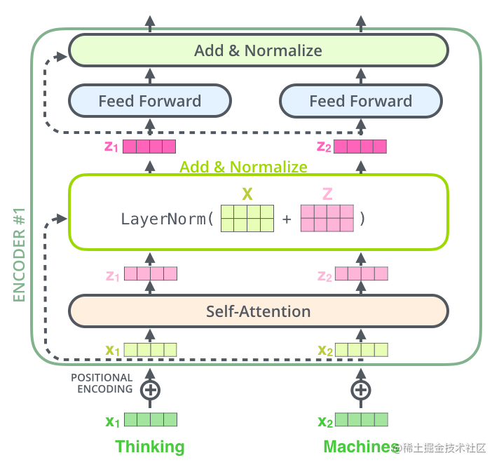
Input word embedding x1 and x2 into Attention to get z1 and z2, then combine x1 and x2 to form matrix X, z1 and z2 form matrix Z, calculate LayerNorm (X+Z), and enter the next layer. The code is implemented as follows:

# 定义层
mta = layers.MultiHeadAttention(4, 10)
ln = layers.LayerNormalization()
# 正向传播
X = tf.random.uniform((3, 10, 5))
Z = mta(X, X)
out = ln(X+Z)
# 输出 (3, 10, 5)
print(out.shape)

（4）Feed Forward

Feed Forward is a simple fully connected layer, but here a single vector is fully connected, that is, each vector z1-zn passes through the Linear layer independently. In addition, the Feed Forward layer has two layers of full connection, first zooming in and then zooming out. The code is as follows:

import keras
from keras import layers
import tensorflow as tf

mta = layers.MultiHeadAttention(4, 10)
ln = layers.LayerNormalization()
# Feed Forward层
ff = keras.Sequential([
    layers.Dense(10, activation='relu'),
    layers.Dense(5)
])
X = tf.random.uniform((3, 10, 5))
Z = mta(X, X)
Z = ln(X+Z)
out = ff(Z)
# 输出 (3, 10, 5)
print(out.shape)

At this point we have explained the various components of the Encoder. Next, implement the TransformerEncoder layer.

3.2 Implementation of Encoder

Now we write the above parts into a TransformerEncoder class, which does not include PositionalEmbedding. The code is as follows:

class TransformerEncoder(layers.Layer):
    def __init__(self, embed_dim, hidden_dim, num_heads, **kwargs):
        super(TransformerEncoder, self).__init__(**kwargs)
        # Multi-Head Attention层
        self.attention = layers.MultiHeadAttention(
            num_heads=num_heads, key_dim=embed_dim
        )
        # Feed Forward层
        self.feed_forward = keras.Sequential([
            layers.Dense(hidden_dim, activation='relu'),
            layers.Dense(embed_dim)
        ])
        # layernorm层
        self.layernorm1 = layers.LayerNormalization()
        self.layernorm2 = layers.LayerNormalization()

    def call(self, inputs, *args, **kwargs):
        # 计算Self-Attention
        attention_output = self.attention(inputs, inputs)
        # 进行第一个Layer & Norm
        ff_input = self.layernorm1(inputs + attention_output)
        # Feed Forward
        ff_output = self.feed_forward(ff_input)
        # 进行第二个Layer & Norm
        outputs = self.layernorm2(ff_input + ff_output)
        return outputs

Now we implement the TransformerEncoder which receives a batch_size × sequence_len × embed_dimtensor and outputs a tensor with the same shape. If it is to be used for sentiment analysis, we can splice global average pooling and fully connected layers behind the output.

3.3 Classification Model

Below we use the previous PositionalEmbedding and TransformerEncoder to implement our text classification network. The code is as follows:

# 超参数
vocab_size = 20000
seq_len = 180
batch_size = 64
hidden_size = 1024
embed_dim = 256
num_heads = 8
# 加载数据
X_train, y_train = load_data()
X_test, y_test = load_data(r'/home/zack/Files/datasets/aclImdb/test')

vectorization = layers.TextVectorization(
    max_tokens=vocab_size, 
    output_sequence_length=seq_len,
    pad_to_max_tokens=True
)
vectorization.adapt(X_train)
X_train = vectorization(X_train)
X_test = vectorization(X_test)
# 构建模型
inputs = layers.Input(shape=(seq_len,))
x = PositionalEmbedding(vocab_size, seq_len, embed_dim)(inputs)
x = TransformerEncoder(embed_dim, hidden_size, num_heads)(x)
x = layers.GlobalAveragePooling1D()(x)
x = layers.Dropout(0.5)(x)
outputs = layers.Dense(1, activation='sigmoid')(x)
model = keras.Model(inputs, outputs)
# 训练
model.compile(loss='binary_crossentropy', metrics=['accuracy'])
model.fit(
    X_train,
    y_train,
    epochs=20,
    batch_size=batch_size,
    validation_data=[X_test, y_test]
)

After final training, the accuracy on the test set is around 85%.