Twitter sentiment analysis about depression
introduce
Depression poses a huge challenge to global public health. Every day, millions of people suffer from depression, and only a small proportion receive appropriate treatment. In the past, doctors typically diagnosed patients using diagnostic criteria to identify depression (such as the DSM-5 Diagnostic Criteria for Depression) through face-to-face conversations. However, previous research has shown that most patients do not seek help from a doctor in the early stages of depression, which leads to a decline in their mental health. On the other hand, many people use social media platforms every day to share their emotions. Since then, there have been numerous studies on the use of social media to predict mental health and physical illnesses such as cardiac arrest, Zika virus, and prescription drug abuse. This study focuses on using social media data to detect depressive thoughts in social media users. Essentially, the study combined text analysis and focused on extracting insights from written communications to draw conclusions about whether the data was related to depressive thoughts.
This project aims to share their feelings about mental health, determine the presence of anxiety and depression, perform EDA analysis on the data set, and perform sentiment analysis on Twitter text.
data
The data is collected in an unsanitized format using the Twitter API. The data has been filtered to retain only English content. It targets users’ mental health classification at the tweet level.
- post_id: ID of the post
- post_created: post creation time
- post_text: Uncleaned tweet text
- user_id: user ID
- followers: number of fans
- friends: number of friends
- favorites: number of collections
- statuses: total number of statuses
- redata: the total number of retweets of the current tweet
- label: label used for classification (1 means depression, 0 means no depression)
The goal of this example is to use monitoring data to estimate a predictive model and determine whether a user suffers from depression.
In other words, we want to build a model that can classify data as "depressed" and "not depressed" based on its content. I can think of many reasons why this kind of thing is so cool. One of the reasons I put forward is that one can judge the psychological state of users based on their emotions and promote related products. For example, people suffering from depression can promote medications. Medication is one of the most effective treatments for depression, so categorizing tweets as "depressed" and "not depressed" is useful for this. The steps for this project are as follows: 1. Initial cleanup of the text. 2. Data visualization. 3. Convert it to format using the "tm" package. 4. Split the data into "training" and "test" sets. 5. Define the "features" of the classification model using the "one-hot encoding" method. 6. Apply the Naive Bayes algorithm to the "training" data in the "e1071" package. 7. Use the model to make predictions from the "test" data.
Data cleaning
Next, download the dataset and read it using the following code:
The first thing I did was cast the "label" field to a factor, rather than a value.
##
## no depression    depression
##         10000         10000
There are 10,000 pieces of depression data and 10,000 pieces of non-depression data
. This second step is a little tricky. I have tried using tidyr and tm packages for text mining applications. They all have built-in functionality for cleaning up regular expressions and other complex content extraction from text data. For some reason I've been having trouble handling certain special characters like non-ASCII or escaped characters. Here, I used a simple gsub() operation to clean out some content from the tweet text.
A “bag-of-words” model treats each tweet as a large bag of words. Using the tm package to organize data, the first thing we need to do is create a corpus. A corpus is a collection of documents. In this case, each tweet is a document.
## <<SimpleCorpus>>
## Metadata:  corpus specific: 1, document level (indexed): 0
## Content:  documents: 20000
Now we have a corpus of 20,000 documents (data).
The tm package has some built-in methods to remove things like punctuation and stop words. We will use these methods to remove some content from the corpus:
## <<SimpleCorpus>>
## Metadata:  corpus specific: 1, document level (indexed): 0
## Content:  documents: 5
##
## [1] just year sinc diagnos anxieti depress today im take moment reflect far ive come sinc
## [2] sunday need break im plan spend littl time possibl
## [3] awak tire need sleep brain idea
## [4] rt sewhq retro bear make perfect gift great beginn get stitch octob sew sale now yay httptco
## [5] hard say whether pack list make life easier just reinforc much still need movinghous anxieti
data visualization
Word clouds provide an intuitive way to visualize the frequency of words in a corpus.
The more frequently a word appears in the corpus, the larger its word size will be in the word cloud.
We can easily create a word cloud by using the wordcloud() function in the wordcloud package.
Drawing words in tweets from people who are not depressed
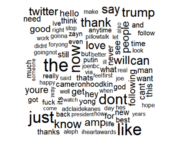
Drawing words in tweets from depressed people

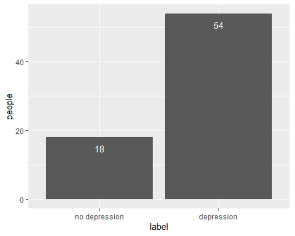
Among the 20,000 tweets, many users tweeted repeatedly. A total of 72 users were surveyed, 54 of whom were depressed and 18 who were not depressed.
document matrix
In the next section, there are a few things to note:
- There exists a TermDocumentMatrix that arranges the terms in the corpus along rows and the documents along columns.
- Then there is a DocumentTermMatrix that arranges the documents along the rows and the terms along the columns.
This application mainly deals with DocumentTermMatrix. This is because when applying the Naive Bayes algorithm, it is convenient to put observations in rows and features (words) in columns.
## [1] 20000 28725
The current document-term matrix contains 28,725 words extracted from 20,000 tweets. These words will be used to decide whether a tweet is positive or negative.
The document-term matrix is 100% sparse, meaning no words are left outside the matrix.
## [1] 20000  1109
## <<DocumentTermMatrix (documents: 10, terms: 15)>>
## Non-/sparse entries: 20/130
## Sparsity           : 87%
## Maximal term length: 7
## Weighting          : term frequency (tf)
## Sample             :
##     Terms
## Docs anxieti come depress diagnos far ive just need sinc take
##   1        1    1       1       1   1   1    1    0    2    1
##   10       0    0       0       0   0   0    0    0    0    0
##   2        0    0       0       0   0   0    0    1    0    0
##   3        0    0       0       0   0   0    0    1    0    0
##   4        0    0       0       0   0   0    0    0    0    0
##   5        1    0       0       0   0   0    1    1    0    0
##   6        0    0       0       0   0   0    0    0    0    0
##   7        0    0       0       0   0   0    0    0    0    0
##   8        0    0       0       0   0   0    0    0    0    0
##   9        0    0       0       0   0   0    0    0    0    1
The regular inspect() method is not very informative. However, if we want to know how often some words or phrases appear in the corpus, one thing we can do is pass the terms as a dictionary to the DocumentTermMatrix() method.
Just to follow up. In the output above, we see that file 1 has 1 occurrence of the phrase "anxiety" and 1 occurrence of "depression". If we look at the raw tweet text dataframe, we can see:
## [1] "Its just over 2 years since I was diagnosed with anxiety and depression Today Im taking a moment to reflect on how far Ive come since"
It's good to take a look at words that appear more than 700 times.
##            word freq
## like       like 1035
## depress depress  953
## just       just  943
## dont       dont  832
## get         get  794
## one         one  746

Model
Naive Bayes is trained on categorical data and converts numerical data into categorical data. We will transform the numeric features by creating a function that converts any non-zero positive value into a "yes" and all zero values into a "no" to state whether a specific term is present in the document.
This routine changes the elements of DocumentTermMatrix from word count to presence/absence. Here are some good open source notes on NLP from a course at Stanford University. Included is some discussion of the binary (Boolean trait) Naive Bayes algorithm.
We now split the dataset into training and testing datasets. We will use 90% of the data for training and the remaining 10% for testing.
##    user  system elapsed
##    0.72    0.01    0.74
Model Evaluation for Naive Bayes
## Confusion Matrix and Statistics
##
##                Reference
## Prediction      no depression depression
##   no depression          1006          0
##   depression                0        970
##
##                Accuracy : 1
##                  95% CI : (0.9981, 1)
##     No Information Rate : 0.5091
##     P-Value [Acc > NIR] : < 2.2e-16
##
##                   Kappa : 1
##
##  Mcnemar's Test P-Value : NA
##
##             Sensitivity : 1.0000
##             Specificity : 1.0000
##          Pos Pred Value : 1.0000
##          Neg Pred Value : 1.0000
##              Prevalence : 0.5091
##          Detection Rate : 0.5091
##    Detection Prevalence : 0.5091
##       Balanced Accuracy : 1.0000
##
##        'Positive' Class : no depression
The Naive Bayes model performed best with 100% accuracy compared to the Support Vector Machine and Random Forest models which were 100% and 100% respectively. Naive Bayes works by assuming that the features of a data set are independent of each other - hence the name Naive.
result
The project classifies tweets based on their text to predict whether they suffer from depression. The accuracy of the Bayesian model on the test set has reached a very good level. Patients used to be lively and cheerful, but their recent tweets have been very depressed, or their status has changed, such as sleep problems and physical problems. Such users may suffer from depression
code
library(tidyverse)
library(ggthemes)
library(e1071) # has the naiveBayes algorithm
library(caret) # good ML package, I like the confusionMatrix() function
library(tm) # for text mining
# Load package
library(wordcloud)
Sys.setenv(LANG="en_US.UTF-8")
###  https://www.kaggle.com/datasets/infamouscoder/mental-health-social-media
data <- read_csv("Mental-Health-Twitter.csv")
data$label <- factor(data$label,levels = c(0,1),
                     labels  = c("no depression","depression"))
table(data$label)

data$post_text <- gsub("[^[:alnum:][:blank:]?&/\\-]", "", data$post_text)
corpus <- Corpus(VectorSource(data$post_text))
corpus
clean.corpus <- corpus %>% tm_map(tolower) %>%
    tm_map(removeNumbers) %>%
    tm_map(removeWords, stopwords()) %>%
    tm_map(removePunctuation) %>%
    tm_map(stripWhitespace)%>%
    tm_map(stemDocument)
inspect(clean.corpus[1:5])
no_depression <- subset(data,label=="no depression")
wordcloud(no_depression$post_text, max.words = 100, scale = c(3,0.5))
depression <- subset(data,label=="depression")
wordcloud(depression$post_text, max.words = 100, scale = c(3,0.5))
df <- data%>%
    group_by(user_id,label)%>%
    count()

ggplot(df, aes(x = label)) +
  geom_bar() +
  geom_text(aes(label = ..count..), stat = "count", vjust = 2, colour = "white")  + ylab("people")
# Create the Document Term Matrix
dtm <- DocumentTermMatrix(clean.corpus)
dim(dtm)
dtm = removeSparseTerms(dtm, 0.999)
dim(dtm)
#Inspecting the the first 10 tweets and the first 15 words in the dataset
inspect(dtm[0:10, 1:15])
data$post_text[1]
freq<- sort(colSums(as.matrix(dtm)), decreasing=TRUE)
wf<- data.frame(word=names(freq), freq=freq)
head(wf)
ggplot(head(wf,10),aes(x = fct_reorder(word,freq),y = freq)) + geom_col() + xlab("word") + ggtitle("Top 10 words in Tweets")
convert_count <- function(x) {
    y <- ifelse(x > 0, 1,0)
    y <- factor(y, levels=c(0,1), labels=c("No", "Yes"))
    y
}
# Apply the convert_count function to get final training and testing DTMs
datasetNB <- apply(dtm, 2, convert_count)