An orthogonal table is a table used in multifactorial experimental designs. It can help us determine the influence of various factors on the results with as few trials as possible, thereby improving the efficiency of experiments. Next, the relevant content of the orthogonal table will be introduced from the following aspects.

1. Basic concept of orthogonal table
Orthogonal table is a special table used in multifactorial experimental design research. According to the orthogonality of the orthogonal table, as few representative combinations as possible can be selected from the comprehensive test, and these combinations have the characteristics of "balanced dispersion, neat and comparable" . "Balanced dispersion" makes the experimental points representative; "neat and comparable" facilitates the analysis of experimental data. Experimenting with the orthogonal table can greatly save the manpower, material resources and time cost of the experiment, and facilitate the determination of the influence of various factors on the experimental results, thereby improving the efficiency of the experiment.
Second, the composition of the orthogonal table
(1) Factors and levels
Before understanding the composition of the orthogonal table, it is necessary to understand the concept of the factors and levels of the orthogonal experiment .
Factor: Refers to the variables in the experiment; such as temperature, time, and catalyst type, a total of three factors.
Level: Refers to the different values of the experimental factors; for example, the temperature is divided into 30°C, 50°C, and 80°C, which means that the factor of temperature is three levels.
Usually when describing an orthogonal test, it is directly said that several factors and several levels of orthogonal tests are carried out, such as three factors and three levels of orthogonal tests.
(2) Representation
Orthogonal tables are usually expressed in the form: L_{number of rows}~(number of levels~^{number of factors})

L represents an orthogonal table, and the number of rows represents the number of experiments to be performed; the number of factors represents the number of variables in the experiment, that is, the number of columns in the orthogonal table; the number of levels represents the number of levels of each factor. where number of rows = number of factors * (number of levels - 1) + 1
For example: For example, the orthogonal table L_{9}~(3~^{4}), the number "9" in the lower right corner of L indicates that there are 9 rows, that is, 9 experiments need to be done. The index "4" in brackets means that there are 4 columns, that is, up to 4 factors can be observed. The number "3" in brackets indicates that each factor has 3 levels, that is, the main part of the table only has numbers 1, 2, and 3, representing levels 1, 2, and 3, respectively. If the four-factor and three-level experiment is carried out comprehensively, 3~^{4}=81 experiments are required, while the orthogonal experiment only needs to be carried out 9 times, which greatly increases the experimental efficiency. The four-factor three-level orthogonal design table is shown in the figure below:
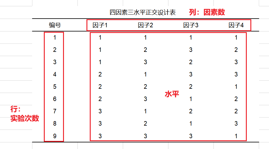
figure 1
When the number of levels of each factor in the orthogonal table is different, it is called a mixed orthogonal table at this time , such as the orthogonal table L_{8}~(4~^{1}2~^{4}), expressed in Of the 5 columns in this table, 1 column is 4 levels and 4 columns are 2 levels.
3. Properties of Orthogonal Tables
Orthogonal table must satisfy the following two properties at the same time:
① Neat comparability - the number of occurrences of different numbers in each column is equal
That is, the number of occurrences of each level of each factor is exactly the same. Since each level of each factor in the experiment has the same probability of participating in the experiment as each level of other factors, this ensures that the interference of other factor levels is excluded to the greatest extent in each level, and the most effective Comparison, and then it is easy to find the optimal experimental conditions.
For example, in the four-factor three-level orthogonal test table in Figure 1, the numbers 1, 2, and 3 appear three times in each column, which satisfies the orderly comparability.
②Equilibrium dispersibility - the number arrangement of any two columns is complete and balanced
That is to say, the horizontal collocation of any two factors is exactly the same (in any pair of numbers formed by two horizontal columns, the number of occurrences of each pair of numbers is equal). This ensures that the experimental conditions are evenly dispersed in the complete combination of factor levels and have strong representativeness.
For example, in the three-level test in Figure 1, there are 9 pairs of numbers in any two columns, (1,1) (1,2) (1,3) (2,1) (2,2) (2,3) ( 3,1) (3,2) (3,3), and each pair has an equal number of occurrences.
Fourth, the generation of orthogonal tables
The design of the orthogonal table requires the knowledge of combinatorics and probability. Manually designing the orthogonal table is time-consuming and laborious. At present, many software can generate the orthogonal table online. Next, we will introduce how to use the online data analysis software SPSSAU to quickly generate the orthogonal table. .
SPSSAU provides two ways to generate an orthogonal table, as follows:
(1) Automatically generate an orthogonal table
In the [Experiment/Medical Research] module, select the analysis method [Orthogonal Test], select the number of factors (factors) and the number of levels in turn, and click Start Analysis to get the closest orthogonal table. Taking three factors and three levels as an example, the operation is as follows:
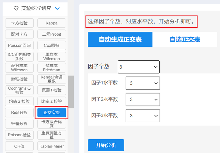
figure 2
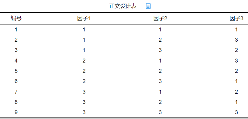
At this time, SPSSAU outputs a three-factor three-level orthogonal design table as shown below:
(2) Optional orthogonal table
If you know what kind of orthogonal table you need, you can generate it by choosing an orthogonal table. You can drop down to select common orthogonal tables:

image 3
Or enter the ID of the orthogonal table. Currently, SPSSAU provides a total of 183 orthogonal tables. You can click the "Download button" to view the manual of the SPSSAU orthogonal table. The display part is as follows:

Figure 4
(3) Orthogonal table modification
After the orthogonal table is automatically provided by the software, it may not fully meet the expectations, so the following processing is required.
①If there is an excess factor, just delete it directly; since any two columns of the orthogonal table satisfy the orthogonality, deleting a certain column will not affect it.
②'Quasi-level method': If the number of levels of a certain factor is more than expected, for example, factor 1 of the generated orthogonal table has 5 levels, but only 4 levels are needed; then at this time, the extra number 5 (the 5th Level), just replace and fill with any one or more of the other 4 levels. This treatment is called 'quasi-level method'. The "quasi-horizontal method" is very common in the transformation of the orthogonal table, but after the "quasi-horizontal method", it may no longer have the characteristics of the orthogonal table, which is very normal;
③'Combined method': For example, consider 2 levels, 4 levels, 8 levels; it is not necessary to use 2.1.4.1.8.1; but use, for example, L12.2.11 (because there are 16 levels in 2, which can be divided into: 2, 2*2, 2*2*2, 6 factors are shared, and the remaining 5 factors can be deleted directly if not used), the combination method is a skillful operation method for orthogonal table acquisition, and this operation method is Self-processing and selection before the generation of the intersection table, and the "combination method" has no effect on the orthogonality, it is just a technical method of manually selecting the orthogonal table;
④'Parallel method': refers to combining two or more columns into one column, for example, if there are two factors, one of which is 2 levels and the other is 3 levels; the combination of two factors becomes 2*3=6 levels ;'Parallel method' is a skillful way to select the orthogonal table independently and manually, and the orthogonality still exists after the 'parallel method'.
5. Orthogonal experiment design and analysis steps
The usual steps for designing and analyzing multivariate orthogonal experiments are as follows:
①Determination of factors and levels (related to experimental design);
② Use software to generate corresponding orthogonal table (SPSSAU can quickly generate orthogonal table);
③ Orthogonal test is carried out according to the orthogonal table, and the test result is obtained;
④ Use range analysis or variance analysis to analyze the test to obtain the optimal test conditions.