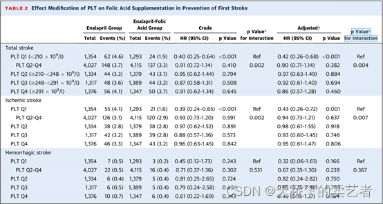
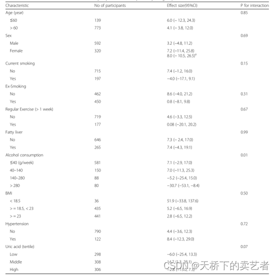
The interaction effect (p for Interaction) can be regarded as a nirvana in SCI articles, and it almost always appears in high-scoring SCIs, because dividing the population into subgroups and then performing statistics can enhance the reliability of the results of the article. Today
we Use R language to draw a table like the one above, continue to use our premature birth data, let's import the data first
bc<-read.csv("E:/r/test/zaochan.csv",sep=',',header=TRUE)
bc <- na.omit(bc)
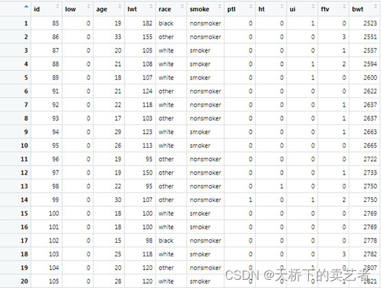
This is the data about premature low birth weight infants (official account reply: premature birth data, this data can be obtained), and the infants below 2500g are considered low birth weight infants. The data is interpreted as follows: low is a premature low birth weight baby less than 2500g, age is the age of the mother, lwt is the last menstrual weight, race is race, smoke is smoking during pregnancy, ptl is history of premature birth (count), ht is history of hypertension, ui is uterine allergy, ftv is early pregnancy Number of doctor visits
bwt Newborn weight value.
We first convert the categorical variables into factors
bc$race<-ifelse(bc$race=="black",1,ifelse(bc$race=="white",2,3))
bc$smoke<-ifelse(bc$smoke=="nonsmoker",0,1)
bc$low<-factor(bc$low)
bc$race<-factor(bc$race)
bc$ht<-factor(bc$ht)
bc$ui<-factor(bc$ui)
Suppose we want to study the effect of maternal age on the relationship between preterm birth, we need to understand the interaction of age and preterm birth among different races.
First divide the age into 3 groups of data
dat1<-subset(bc,bc$race==1)
dat2<-subset(bc,bc$race==2)
dat3<-subset(bc,bc$race==3)
Use these 3 data to build a model respectively. Note that the model does not have the indicator of race
f1<-glm(low~age + lwt + smoke + ptl + ui + ftv, data=dat1,
    family=binomial(link = "logit"))
f2<-glm(low~age + lwt + smoke + ptl + ui + ftv, data=dat2,
        family=binomial(link = "logit"))
f3<-glm(low~age + lwt + smoke + ptl + ui + ftv, data=dat3,
        family=binomial(link = "logit"))
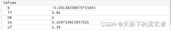
Next, we need to extract the coefficients for each model, we first extract the model f1
b<-summary(f1)$coeff[2,1]#提取系数
se<-summary(f1)$coeff[2,2]#提取标准误
OR<-round(exp(b),2)
ll<-round(exp(b-1.96*se),2)
ul<-round(exp(b+1.96*se),2)
Next, we need to perform the same extraction coefficients for other models. Here I write it as a loop to run. First, set an output function.
jj<-function(data) {


  dat<-data
  fit<-glm(low~age + lwt + smoke + ptl + ui + ftv, data=dat,
           family=binomial(link = "logit"))
  b<-summary(fit)$coeff[2,1]#提取系数
  se<-summary(fit)$coeff[2,2]#提取标准误
  OR<-round(exp(b),3)
  ll<-round(exp(b-1.96*se),3)
  ul<-round(exp(b+1.96*se),3)
  d<-data.frame(OR,ll,ul)
}
Combine 3 data into a list
dt<-list(dat1,dat2,dat3)
Use the sapply function to run
out<-sapply(dt,jj)
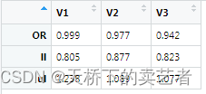
Need to transpose the generated result
out1<-as.data.frame(t(out))
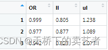
In this way, the result OR value and credible interval are generated. The P value of the interaction effect needs to be calculated separately. I will not demonstrate it here. If you are interested, read my previous articles. My P value here is 0.7358
p<-0.7358
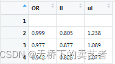
Next, set up the table, now add a row of empty values
out2<-rbind(c("","",""),out1)
Put in our result and rename
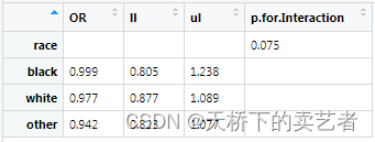
out2$p.for.Interaction<-c(0.075,"","","")
rownames(out2)<-c("race","black","white","other")
Final result display