As in many fields, there are currently two directions of work in deep learning. One is to find more powerful, but also more complex model networks and experimental methods, with the aim ofImproving the performance (accuracy) of deep neural networks, this type of work is mainly done by researchers (academics) .Real-time requirements of complex networksAnother direction of work was born, that is, to study how to implement the research members of scientific researchers into actual hardware and application scenarios, and to ensure that the algorithm is stable and efficient. This type of personnel is the so-called engineering school .
This article sorts out some of the classic CNN evolution structures and its core ideas in the former.
1998 LeNet-5
Y.Lecun original link Gradient-Based Learning Applied to Document Recognition
The structure diagram of LeNet-5 is as follows
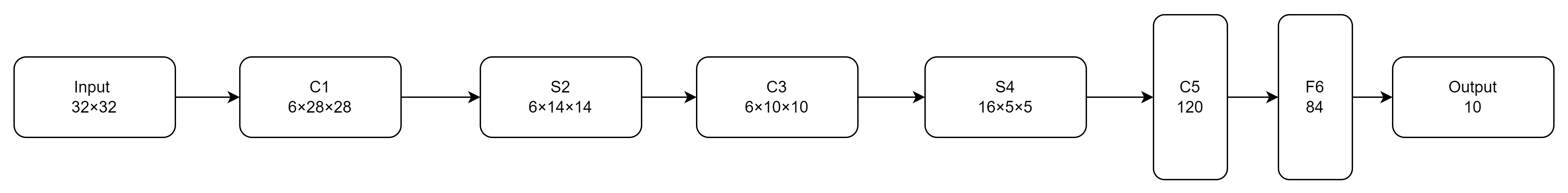
The LeNet-5 network has 7 layers, does not contain input, and each layer contains trainable parameters. Each layer has multiple FeatureMaps, each FeatureMap extracts a feature of the input through a convolution filter, and each FeatureMap has multiple neurons. (For the specific principle, please refer to the analysis of multi-layer perceptron and CNN operator in the previous blog)
Although LeNet-5 is simple, it contains the basic modules of deep learning, namely convolutional layer, pooling layer and fully connected layer . It is a very efficient convolutional neural network for handwritten character recognition.
2012AlexNet
Alex Krizhevsky original link ImageNet Classification with Deep Convolutional Neural Networks
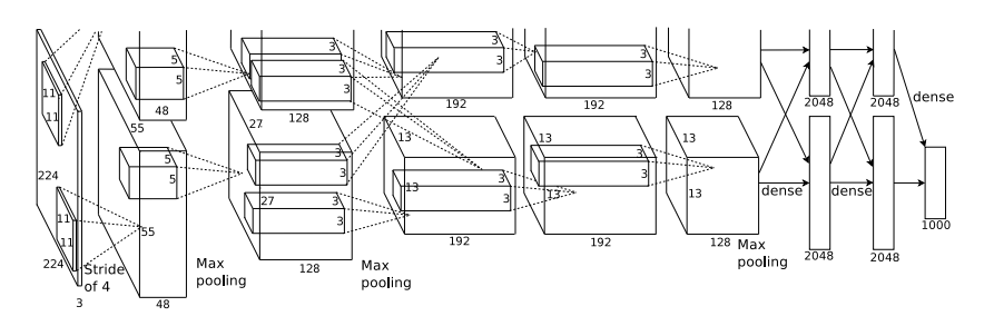
AlexNet is the champion of ILSVRC in 2012. In the original architecture, there are two parallel processing pipelines to allow two GPUs to work together to build training models with faster computing speed and memory sharing. The architecture divided by GPU has less weight because not all layers are interconnected, and reducing some interconnections can reduce the communication time between processors, which can help improve efficiency.
Compared with LeNet, the main innovations of AlexNet are:
- ReLU is used : ReLU is different from Sigmoid. This function is a non-saturated function, which successfully solves the gradient dispersion problem of Sigmoid when the network is deep (gradient dispersion, the derivative value of the Sigmoid function is close to 0 when saturated).
- Use Dropout to avoid over-fitting of the model: Use Dropout to randomly ignore some neurons during training to avoid over-fitting of the model.
- All use max pooling instead of the previous average pooling.
- Realize data enhancement : Randomly cut out a 224×224 size area (and a horizontally flipped mirror image) from the 256×256 original image, which is equivalent to enhancing (256-224)×(256-224)×2=2048 times the data quantity. After the original image is augmented with data, it reduces overfitting and improves the generalization ability.
It is worth noting that Clarifai, a variant of ZFNet in 2013, was the winner of ILSVRC in 2013. There is not much difference between ZFNet and AlexNet in terms of architecture. The main change is the difference in the choice of hyperparameters , such as the step size of the initial filter is changed from 4 to 2, and more filters are used in the third, fourth and fifth convolutional layers. device etc. This reminds us: small details matter when working with deep learning algorithms. ZFNet reduced the top-5 error rate from AlexNet's 15.4% to 14.8%, and after Clarifai further increased the width/depth, the top-5 error rate decreased to 11.1%.
VGG and GoogleLeNet in 2014
VGG was the top performer at ISLVRC 2014, but it wasn't the winner. The winner is GoogleNet, which has a top-5 error rate of 6.7%, while VGG has an error rate of 7.3%.
VGG
Karen Simonyan original link Very Deep Convolutional Networks for Large-Scale Image Recognition
VGG embodies the trend of increasing network depth . An important innovation of VGG is to reduce the size of the filter. Reducing the size of the filter requires increasing the depth . This is because unless the network is very deep, a small filter can only capture a small area of the image . For example, in a 7×7 input, a single feature captured by 3 consecutive 3×3 convolutions will form a new region. Note that using a single 7×7 filter directly on the input data will also capture the visual features of the 7×7 input region. In the first case we use 3×3×3=27 parameters, while in the second case we use 7×7×1=49 parameters. Therefore, the parameters take up less space when using 3 consecutive convolutions. At the same time, 3 consecutive convolutions can usually capture more interesting and complex features than one convolution, and the activations obtained by one convolution will look like the original edge features, so the network with 7×7 filters will not be able to capture more complex features. Small regions capture complex shapes.

In general, the greater the depth, the stronger the nonlinearity and the stronger the regularization. Deeper networks will have greater nonlinearity due to the presence of more ReLU layers, and greater regularization due to the structure imposed by increased depth on the layers by using repeated combinations of convolutions. Another interesting design of VGG is that the number of filters is usually doubled after each max pooling layer . The idea is to always increase the depth by a factor of 2 whenever the space footprint is reduced by 1/2. This design leads to a certain balance of cross-layer computing and is inherited by some later architectures (such as ResNet).
GoogleLeNet
Christian Szegedy Original link Going deeper with convolutions
GoogleLeNet proposes a new concept called Inception (initial architecture). Inception is a network within a network . The beginning part of GoogleLeNet is very similar to the traditional convolutional network, the key is the middle Inception module. The basic idea of Inception is that the key information in the image can be obtained at different levels of detail . If you use a large filter, you can capture information in larger areas with limited change; if you use a smaller filter, you can capture detailed information in smaller areas. In the Inception layer, previous layers can be convolved in parallel with filters of different sizes (1×1, 3×3, and 5×5), allowing the neural network to flexibly model images at different levels of granularity . And since all filters on the Inception layer are learnable, the neural network can determine which filters have a great influence on the output.

GoogleLeNet consists of 9 Inception modules arranged in sequence, with a total of 22 layers. By choosing different paths, it will be able to represent different spatial regions . For example: passing 4 3×3 filters and 1 1×1 filter will capture a relatively small spatial area, while passing many 5×5 filters will result in a larger space occupation. Objects of different scales are processed with appropriate sizes. The flexibility of this multi-granularity decomposition is realized by the Inception module, and it is also one of the keys to its performance. The middle part of its structure can be referred to as follows

There are also some interesting design improvements in GoogleLeNet, such as
1. Subsequent batch normalization combined with Inception simplifies the network architecture.
2. Use 1×1 convolution to reduce the depth of the feature map, which is called bottleneck convolution . After the bottleneck is applied, since the depth of the layers is reduced, the depth of the feature maps is also reduced eventually, thus saving the computational efficiency of larger convolutions.
3. A single value is created by averaging pooling over the entire spatial region of the final activation atlas without using a fully connected layer, the number of features created in the final layer will be exactly equal to the number of filters. Replacing the fully connected layer with the average pooling layer greatly reduces the parameter occupancy.
It is worth noting that Inception has since become a hot spot for researchers . In the evolved Inception-v4, combined with some ideas in ResNet, a 75-layer architecture was created, achieving an error rate as low as 3.08%! Please note: the human error rate is 5.1% when classifying images in the ImageNet database. Therefore, how to further improve the accuracy of the model in follow-up research has gradually become no longer the focus of attention, and more attention has shifted to how to satisfy complex networks. real-time requirements.
2015 ResNet
Kaiming He Original link Deep Residual Learning for Image Recognition
ResNet uses 152 layers, which at first glance is an order of magnitude more than any other previous architecture that won ILSVRC 2015 and achieved a top-5 error rate of 3.6%, resulting in the first A classifier with human-level performance. The first problem with training such a deep network is that the increase in depth will bring gradient explosion or gradient disappearance (the accumulation of derivative values of multi-layer activation functions will inevitably hinder the reasonable gradient flow), which can be solved by introducing batch normalization . In addition to this, the learning process struggles to converge correctly in a reasonable amount of time after increasing depth, a convergence problem that is also common in networks with complex loss surfaces.
This basic idea arises: Although hierarchical feature engineering is the holy grail of neural network learning, its hierarchical implementation forces all images in an image to require the same level of abstraction. Some concepts can be learned by using shallow networks, while others may require fine-grained connections . When using a very deep network with a fixed depth on all paths to learn concepts, the convergence process will be very slow, many of which can also be learned using shallow architectures. So why not let the neural network decide how many layers to use to learn each feature?
ResNet uses skip connections (Residual, residual) between layers to replicate between layers. Most feedforward networks only contain connections between layer i and layer i+1, while Resnet contains connections between layer i and layer i+r (r>1). An example of such a skip connection that constitutes the basic unit of Resnet is as follows

Introducing a residual module enables efficient gradient flow , as the backpropagation algorithm now has a superhighway to backpropagate gradients using skip connections. In addition, since some layers use strided convolutions to shrink each spatial dimension to 1/2, and use more filters, the depth is increased to 2 times (see the balanced design of cross-layer computation in VGG). In this case, instead of using the identity function directly on the skip connections, a linear projection matrix is applied to adjust the dimensions . The projection matrix defines a set of 1×1 convolution operations with a step size of 2, which reduces the spatial range to 1/2 of the original, and the parameters of the projection matrix need to be learned during the backpropagation process. The figure below shows part of the ResNet architecture, with skip connections represented by solid lines and projection matrix connections represented by dotted lines

In residual learning, the shortest path can achieve the maximum learning, while the longer path can be regarded as the residual contribution. This gives the learning algorithm the flexibility to choose an appropriate nonlinearity for a particular input , with learning along longer paths being a fine-tuning of easy learning along shorter paths. ResNet has also produced more variants, such as wide residual network, highway network and DenseNet.
SENet 2017
Jie Hu Original text link SENet
SENet was the champion of the 2017 ILSVRC finale, reducing the error rate to 2.251%! Unlike previous studies that focused on how to improve network performance through spatial dimensions (such as deepening and widening the network), SENet improves network performance by modeling channel relationships. The main point is to automatically obtain the importance of each channel by means of learning, and then improve useful features and suppress features that are not very useful for the current task according to this importance .
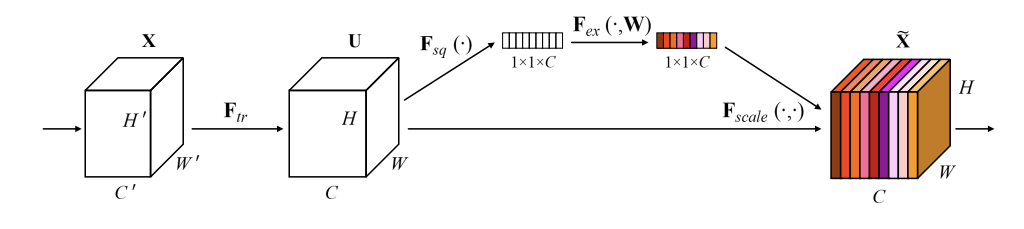
The key operations in SENet are Squeeze (compression) and Excitation (excitation) operations, which is also the origin of its name.
- S: Perform feature compression along the spatial dimension, turning each two-dimensional feature channel into a real number. This real number has a global receptive field to some extent , and the output dimension matches the number of input feature channels.
- E: It is a mechanism similar to the gate in the recurrent neural network, which generates weights for each channel through parameters , where the parameters are learned to explicitly model the correlation between feature channels.
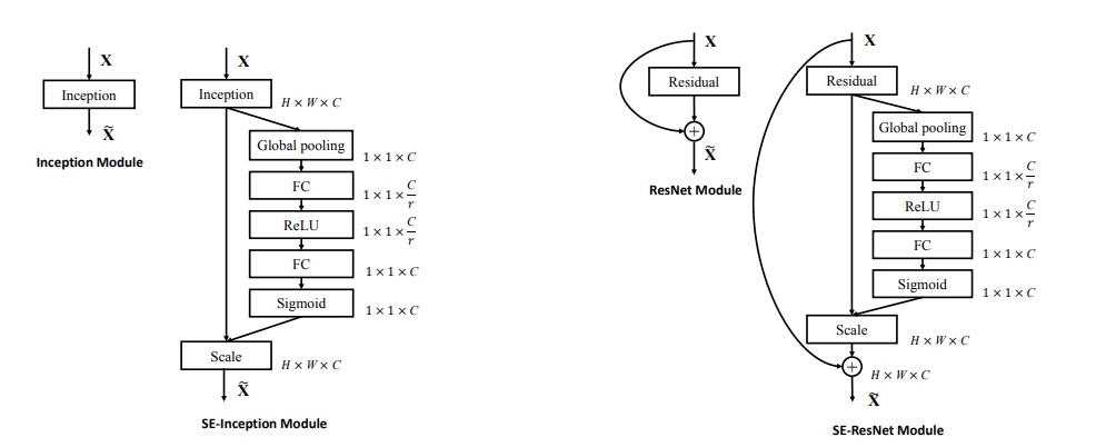
The SE module first performs the Squeeze operation on the feature map obtained by the convolution to obtain the channel-level global features, and then performs the Excitation operation on the global features to learn the relationship between each channel to obtain the weights of different channels. Finally, the Reweight is multiplied by the original features. Figure to get the final features. In essence, the SE module performs attention or gating operations on the channel dimension. This attention mechanism allows the model to pay more attention to the channel features with the most information and suppress those unimportant channel features.
It is worth noting that the flexibility of the SE module allows it to be directly applied to existing network structures , such as Inception and ResNet. Moreover, after the introduction of the SE module, the amount of calculation brought about by the increase in the number of parameters is not significant, but it can effectively improve the performance.
Chapter 8 of "Practical Principles, Architecture and Optimization of Deep Neural Networks on Mobile Platforms" Lu Yusheng Machinery Industry Press
"Neural Networks and Deep Learning" Chapter 8 Charu C.Aggarwal Machinery Industry Press
SENet reference blog post: https://blog.csdn .net/gaoxueyi551/article/details/120233959 and https://zhuanlan.zhihu.com/p/65459972/