Neural network itself consists of a series feature extractor, the ideal feature map should be sparse and contain typical local information. By model visualization can have some intuitive understanding and help us debug models, such as: feature map and very close to the original, it does not explain what features to learn; or it is almost a solid color chart, indicating that it is too sparse, probably we feature several map too much (feature_map lot number also reflects the convolution kernel is too small). Visualization there are many, such as: feature map visualization, visual weight and so on, in my feature map visualization example.
Model visualization
Keras do with the experiment, the following figures as input:
- Enter the picture

- feature map visualization
Take the first layer of the network 15, each take the first three feature map.
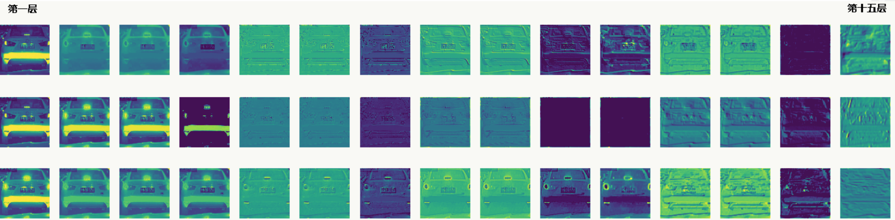
From left to right, you can see the whole feature extraction process, some isolated background, some contour extraction, to extract some color, but can also be found between the two layers 10 and 11 feature map is a solid, this may the number of layers feature map a little bit more, otherwise affect halo car for the feature map in halo can also see more obvious.
- Hypercolumns
We usually last a neural network layer as a fully connected fc entire image feature representation, but this representation may be too coarse (from the above feature map visualization can see it), can not accurately characterize the local space, and the network wherein the first layer are too precise space, lack of semantic information (such as the back color, contour, etc.), then the paper " Hypercolumns Segmentation for Object Localization and Fine-grained " a novel feature representation: Hypercolumns-- the one pixel is defined as a vector of all hypercolumn cnn units should activate the output value of the pixel positions composition), a good tradeoff two previous problems, as shown in FIG intuitively:

把汽车第1、4、7层的feature map以及第1, 4, 7, 10, 11, 14, 17层的feature map分别做平均,可视化如下:

代码实践
  1 # -*- coding: utf-8 -*-
  2 from keras.applications import InceptionV3
  3 from keras.applications.inception_v3 import preprocess_input
  4 from keras.preprocessing import image
  5 from keras.models import Model
  6 from keras.applications.imagenet_utils import decode_predictions
  7 import numpy as np
  8 import cv2
  9 from cv2 import *
 10 import matplotlib.pyplot as plt
 11 import scipy as sp
 12 from scipy.misc import toimage
 13
 14 def test_opencv():
 15     # 加载摄像头
 16     cam = VideoCapture(0)  # 0 -> 摄像头序号,如果有两个三个四个摄像头,要调用哪一个数字往上加嘛
 17     # 抓拍 5 张小图片
 18     for x in range(0, 5):
 19         s, img = cam.read()
 20         if s:
 21             imwrite("o-" + str(x) + ".jpg", img)
 22
 23 def load_original(img_path):
 24     # 把原始图片压缩为 299*299大小
 25     im_original = cv2.resize(cv2.imread(img_path), (299, 299))
 26     im_converted = cv2.cvtColor(im_original, cv2.COLOR_BGR2RGB)
 27     plt.figure(0)
 28     plt.subplot(211)
 29     plt.imshow(im_converted)
 30     return im_original
 31
 32 def load_fine_tune_googlenet_v3(img):
 33     # 加载fine-tuning googlenet v3模型,并做预测
 34     model = InceptionV3(include_top=True, weights='imagenet')
 35     model.summary()
 36     x = image.img_to_array(img)
 37     x = np.expand_dims(x, axis=0)
 38     x = preprocess_input(x)
 39     preds = model.predict(x)
 40     print('Predicted:', decode_predictions(preds))
 41     plt.subplot(212)
 42     plt.plot(preds.ravel())
 43     plt.show()
 44     return model, x
 45
 46 def extract_features(ins, layer_id, filters, layer_num):
 47     '''
 48     提取指定模型指定层指定数目的feature map并输出到一幅图上.
 49     :param ins: 模型实例
 50     :param layer_id: 提取指定层特征
 51     :param filters: 每层提取的feature map数
 52     :param layer_num: 一共提取多少层feature map
 53     :return: None
 54     '''
 55     if len(ins) != 2:
 56         print('parameter error:(model, instance)')
 57         return None
 58     model = ins[0]
 59     x = ins[1]
 60     if type(layer_id) == type(1):
 61         model_extractfeatures = Model(input=model.input, output=model.get_layer(index=layer_id).output)
 62     else:
 63         model_extractfeatures = Model(input=model.input, output=model.get_layer(name=layer_id).output)
 64     fc2_features = model_extractfeatures.predict(x)
 65     if filters > len(fc2_features[0][0][0]):
 66         print('layer number error.', len(fc2_features[0][0][0]),',',filters)
 67         return None
 68     for i in range(filters):
 69         plt.subplots_adjust(left=0, right=1, bottom=0, top=1)
 70         plt.subplot(filters, layer_num, layer_id + 1 + i * layer_num)
 71         plt.axis("off")
 72         if i < len(fc2_features[0][0][0]):
 73             plt.imshow(fc2_features[0, :, :, i])
 74
 75 # 层数、模型、卷积核数
 76 def extract_features_batch(layer_num, model, filters):
 77     '''
 78     批量提取特征
 79     :param layer_num: 层数
 80     :param model: 模型
 81     :param filters: feature map数
 82     :return: None
 83     '''
 84     plt.figure(figsize=(filters, layer_num))
 85     plt.subplot(filters, layer_num, 1)
 86     for i in range(layer_num):
 87         extract_features(model, i, filters, layer_num)
 88     plt.savefig('sample.jpg')
 89     plt.show()
 90
 91 def extract_features_with_layers(layers_extract):
 92     '''
 93     提取hypercolumn并可视化.
 94     :param layers_extract: 指定层列表
 95     :return: None
 96     '''
 97     hc = extract_hypercolumn(x[0], layers_extract, x[1])
 98     ave = np.average(hc.transpose(1, 2, 0), axis=2)
 99     plt.imshow(ave)
100     plt.show()
101
102 def extract_hypercolumn(model, layer_indexes, instance):
103     '''
104     提取指定模型指定层的hypercolumn向量
105     :param model: 模型
106     :param layer_indexes: 层id
107     :param instance: 模型
108     :return:
109     '''
110     feature_maps = []
111     for i in layer_indexes:
112         feature_maps.append(Model(input=model.input, output=model.get_layer(index=i).output).predict(instance))
113     hypercolumns = []
114     for convmap in feature_maps:
115         for i in convmap[0][0][0]:
116             upscaled = sp.misc.imresize(convmap[0, :, :, i], size=(299, 299), mode="F", interp='bilinear')
117             hypercolumns.append(upscaled)
118     return np.asarray(hypercolumns)
119
120 if __name__ == '__main__':
121     img_path = '~/auto1.jpg'
122     img = load_original(img_path)
123     x = load_fine_tune_googlenet_v3(img)
124     extract_features_batch(15, x, 3)
125     extract_features_with_layers([1, 4, 7])
126     extract_features_with_layers([1, 4, 7, 10, 11, 14, 17])
还有一些网站做的关于CNN的可视化做的非常不错,譬如这个网站:http://shixialiu.com/publications/cnnvis/demo/,可以在训练的时候采取不同的卷积核尺寸和个数对照来看训练的中间过程。
Tensorflow的可视化
Tensorboard是Tensorflow自带的可视化模块,可以通过Tensorboard直观的查看神经网络的结构,训练的收敛情况等。要想掌握Tensorboard,我们需要知道一下几点:
- 支持的数据形式
- 具体的可视化过程
- 如何对一个实例使用Tensorboard
数据形式
(1)标量Scalars
(2)图片Images
(3)音频Audio
(4)计算图Graph
(5)数据分布Distribution
(6)直方图Histograms
(7)嵌入向量Embeddings
可视化过程
(1)建立一个graph。(2)确定在graph中的不同节点设置summary operations。(3)将(2)中的所有summary operations合并成一个节点,运行合并后的节点。(4)使用tf.summary.FileWriter将运行后输出的数据都保存到本地磁盘中。(5)运行整个程序,并在命令行输入运行tensorboard的指令,打开web端可查看可视化的结果
使用Tensorborad的实例
这里我就不讲的特别详细啦,如果用过Tensorflow的同学其实很好理解,只需要在平时写的程序后面设置summary,tf.summary.scalar记录标量,tf.summary.histogram记录数据的直方图等等,然后正常训练,最后把所有的summary合并成一个节点,存放到一个地址下面,在linux界面输入一下代码:
tensorboard --logdir=‘存放的总summary节点的地址’
然后会出现以下信息:
1 Starting TensorBoard 41 on port 6006 2 (You can navigate to http://127.0.1.1:6006)
将http://127.0.1.1:6006在浏览器中打开,就可以看到web端的可视化了
