Open source Python microgrid simulator pymgrid for artificial intelligence research (introduction)

pymgrid is an open source Python library for simulating the three-level control of microgrids, allowing users to create or self-select microgrids. These microgrids can be controlled using custom algorithms or one of the control algorithms included in pymgrid (rule-based control and model predictive control).

pymgrid also provides an environment counterpart to the OpenAI Gym API, providing continuous and discrete action space environments for use with reinforcement learning algorithms to train control algorithms.

pymgrid tries to provide a simple, intuitive API that allows users to focus on their specific application.

1. Open source Python microgrid simulator pymgrid for artificial intelligence research

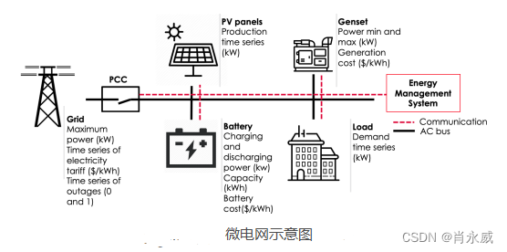
Microgrids, independent grids that can be disconnected from the main grid, have the potential both to mitigate climate change by reducing carbon dioxide emissions and to adapt to climate change by improving infrastructure resilience. Due to their distributed nature, microgrids are often unique; therefore, the control of these systems is non-trivial. While microgrid simulators exist, many are limited in scope and the variety of microgrids that can be simulated. We present pymgrid, an open-source Python package for generating and simulating a large number of microgrids, and the first open-source tool that can generate more than 600 different microgrids. pymgrid abstracts most of the domain expertise, allowing users to focus on the control algorithm. In particular, pymgrid is a reinforcement learning (RL) platform that includes the ability to model microgrids as Markov decision processes. pymgrid also introduces two precomputed lists of microgrids, designed to allow research reproducibility in microgrid settings.

1.1. Overview of pymgrid

pymgrid consists of three main components: a data folder containing load and photovoltaic generation time series for a "seed" microgrid, a microgrid generator class called MicrogridGenerator, and a microgrid simulator class called Microgrid.

1.1.1. Datasets

To easily generate microgrids, pymgrid provides load and photovoltaic generation datasets. Load data comes from DOE OpenEI, based on TMY3 weather data; photovoltaic data is also based on TMY3, provided by DOE/NREL/ALLIANCE. These datasets contain load and photovoltaic files of five cities, each city is in a different climate zone of the United States, the time series is one year, the time step is one hour, and a total of 8760 data points.

1.1.2. Microgrid

This class contains a complete implementation of a microgrid, including time series data and a specific size of the microgrid. Microgrid implements three types of functions: control loops, two benchmark algorithms, and utility functions.

Some functions are required to interact with Microgrid objects. The function run() is used to advance one time step, it takes the control dictionary as parameter and returns the updated state of the microgrid. The control dictionary centralizes all the electrical commands that need to be delivered to the microgrid to operate each generating device at each time step. Once the microgrid reaches the last time step of the data, its done parameter will be passed as True. The function reset() can be used to reset the microgrid to its initial state, clear the tracking data structure and reset the time step. Once a control operation is applied to the microgrid, it checks the function to ensure that the command complies with the microgrid constraints.

For reinforcement learning benchmarks and machine learning more generally, another additional function is useful, train_test_split() allows the user to split a dataset into two parts, a training set and a test set. User can also use reset() to go from training set to testing set, use testing=True parameter in reset function. An example is provided in the list.

1.1.3. MicrogridGenerator类

MicrogridGenerator contains functions to generate a list of microgrids. For each requested microgrid, the process is as follows. First, the maximum power of the load is randomly generated. A load file is then randomly selected and scaled to the previously generated values. The next step is to automatically and randomly select the architecture of the microgrid. Photovoltaics and batteries are always there, this may evolve as we add more components - we randomly choose whether to have a diesel generator (genset), grid, no grid or weak grid (grid-connected system with frequent blackouts). We also implement back-up generators in case of a weak grid; electricity rates are chosen randomly if there is a grid or a weak grid. Electricity rates were generated by MicrogridGenerator and are based on commercial rates in California and France.

Once the architecture has been selected, the microgrid needs to be sized. First, the PV penetration (defined by Hoke et al. [2012] as load maximum power/PV maximum power) needs to be calculated and used to randomly scale the selected PV curve. The size of the generated grid is guaranteed to be greater than the maximum load, and the power generation equipment provides enough power to meet the peak load demand. Finally, the battery is capable of providing power for three to five hours under an average load.

MicrogridGenerator will create a Microgrid object once the different components are selected and adjusted. Repeat this process to generate as many microgrids as the user requests.

Overall, using five load files, five PV files, two electricity tariffs, three grid types, and binary generator selections, the model can generate over 600 different microgrids—not even taking into account possible different PV penetrations. The number of transmittance levels.

1.2. Benchmarks and Discussion

In addition to the above features, we also propose two standard microgrid lists: pymgrid10 and pymgrid25, which contain 10 and 25 microgrids, respectively. pymgrid10 is designed as a first dataset for beginners. It contains 10 microgrids with the same architecture (PV+Battery+Generator), mainly aimed at gaining an intuition about the simulated situation. In pymgrid25, more than 25 microgrids of all possible architectures can be found. Four of these microgrids have generators only, three have generators and a grid, nine have grids only, and nine have generators and a weak grid. Since we propose these collections of microgrids as a standardized test set, we also implement a set of control algorithms as a benchmark comparison. Specifically, we implement four algorithms: rule-based control, model predictive control (MPC), Q-learning, and decision tree (DT)-augmented Q-learning. By examining the results, we see that MPC can be considered almost optimal when it has perfect predictions, while RBC can be considered a lower bound because it gives the performance achievable by simple algorithms.

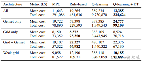
As can be seen from the table above, the performance of the algorithms varies greatly. Q-learning underperforms; however, Q-learning augmented with decision trees outperforms RBC—the average cost of RBC is about 44% higher than DT-augmented Q-learning—while most of the difference occurs in edge cases, where RBC's Performs poorly because of lack of algorithmic complexity. While Q-learning with augmented decision trees may perform well, it must use discrete action spaces, a requirement that reduces the range of actions that a Q-learner can learn, and makes it difficult to ensure that all possible actions are considered in any given discrete action space. action. Across 6 microgrids, RBC outperforms Q-learning augmented with decision trees; this suggests that DT Q-learning may not consistently exceed an acceptable performance lower bound. This problem typically arises in grid-only or microgrids with grid and gensets.

While the difference between Q-learning and MPC augmented with decision trees often appears insignificant, it is important to remember that these 25 microgrids were loaded in the megawatt range; thus, a 13% difference could result in a $40 million additional cost. To combat climate change and integrate more renewable energy, the technology will need to scale up beyond the thousands of systems deployed. Improving controller performance by a few percent can significantly reduce operating costs, increasing the importance of improving controller performance. Reinforcement learning is a promising solution to achieve this goal.

1.3. Conclusions and future work

pymgrid is a Python package that allows researchers to generate and simulate large numbers of microgrids and provides an environment for applications in reinforcement learning research. We establish standard microgrid scenarios for algorithm comparison and reproducibility, and provide performance baselines using classical control algorithms and reinforcement learning. To improve reinforcement learning-based microgrid controllers, a universal and adaptable benchmark simulator is crucial, and pymgrid plays this role. A promising new avenue is to exploit data generated from multiple microgrids to increase performance or adaptability.

Future plans include adding a broader suite of benchmark algorithms, including the latest reinforcement learning methods. We also plan to allow for the addition of other microgrid components, more complex application scenarios, and finer temporal resolution. In addition, we hope to add the function of real-time data acquisition. Finally, functionality on CO2 use and data is extremely valuable for users to control carbon efficiency, while also allowing users to consider the role carbon taxes may play in future energy generation.

2. Install pymgrid

pip install

pip install -i https://pypi.tuna.tsinghua.edu.cn/simple pymgrid

Installation requirements and dependencies

• python>=3.6
• Install dependencies:
  pandas,
  numpy,
  cvxpy,
  statsmodels,
  matplotlib,
  plotly,
  cufflinks,
  gym,
  tqdm,
  pyyaml

Download the source code and install
https://github.com/Total-RD/pymgrid.git

# 进入pymgrid工程根目录下：
pip install -i https://pypi.tuna.tsinghua.edu.cn/simple .

3. Quick start

Define a simple microgrid, create operations that control it, and read the results. A microgrid can be defined by defining a set of modules and then passing them to the microgrid constructor, or through a YAML configuration file.

3.1. Define Microgrid

Define some components of the microgrid. We will define two batteries, one fast charging with a capacity of 100 kWh and one slow charging but with a capacity of 1000 kWh.

import numpy as np
import pandas as pd
np.random.seed(0)
from pymgrid import Microgrid
from pymgrid.modules import (
    BatteryModule,
    LoadModule,
    RenewableModule,
    GridModule)

small_battery = BatteryModule(min_capacity=10,
                              max_capacity=100,
                              max_charge=50,
                              max_discharge=50,
                              efficiency=0.9,
                              init_soc=0.2)

large_battery = BatteryModule(min_capacity=10,
                              max_capacity=1000,
                              max_charge=10,
                              max_discharge=10,
                              efficiency=0.7,
                              init_soc=0.2)

Random data defines loads and photovoltaic (pv) modules, for example, defines 90 days of solar power generation data in hours.

load_ts = 100+100*np.random.rand(24*90) # random load data in the range [100, 200].
pv_ts = 200*np.random.rand(24*90) # random pv data in the range [0, 200].

load = LoadModule(time_series=load_ts)
pv = RenewableModule(time_series=pv_ts)

Finally, we define an external grid to fill any energy gaps. Grid time series must contain three or four columns. The first three represent grid power purchase price, on-grid power price and carbon dioxide production per kWh. If a fourth column is present, it indicates grid status (as a boolean); if absent, the grid is assumed to be always up and running.

grid_ts = [0.2, 0.1, 0.5] * np.ones((24*90, 3))

grid = GridModule(max_import=100,
                  max_export=100,
                  time_series=grid_ts)

Based on the above data, construct a microgrid and use 'pv' to define photovoltaic power generation. By default, a balancing module is added to track any unmet demand or excess production. (Can be disabled with unbalanced_energy_module=False, but not recommended)

A printout of the microgrid will tell us what modules are included in the microgrid.

modules = [
    small_battery,
    large_battery,
    ('pv', pv),
    load,
    grid]

microgrid = Microgrid(modules)
print(microgrid)

output:

Microgrid([load x 1, pv x 1, balancing x 1, battery x 2, grid x 1])

We can access modules in the microgrid by name or key:

print(microgrid.modules.pv)
print(microgrid.modules.grid is microgrid.modules['grid'])

3.2. Control microgrid

You must control the microgrid through the actions of each controllable module. Fixed modules are stored in the property microgrid.controlleble:

microgrid.controllable

	{
	  "battery": "[BatteryModule(min_capacity=10, max_capacity=100, max_charge=50, max_discharge=50, efficiency=0.9, battery_cost_cycle=0.0, battery_transition_model=None, init_charge=None, init_soc=0.2, initial_step=0, raise_errors=False), 
	               BatteryModule(min_capacity=10, max_capacity=1000, max_charge=10, max_discharge=10, efficiency=0.7, battery_cost_cycle=0.0, battery_transition_model=None, init_charge=None, init_soc=0.2, initial_step=0, raise_errors=False)]",
	  "grid": "[GridModule(max_import=100, max_export=100)]"
	}

Our "Load", "Battery" and "Grid" modules are fixed.

We can also see to which modules we need to pass actions by getting empty actions from the microgrid. Here, all None values ​​must be replaced to pass this action as control.

print(microgrid.get_empty_action())

Reset the microgrid, then check its current state.

microgrid.reset()
microgrid.state_series()

Run a random step.

microgrid.run(microgrid.sample_action())
microgrid.current_step
# 查看一步后的状态
# microgrid.state_series()

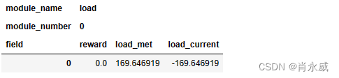
We will try to use available renewable energy and then discharge the battery to meet the load demand of 169.646919. For the battery we will try to generate low excess load and maximum output.

load = -1.0 * microgrid.modules.load.item().current_load
pv = microgrid.modules.pv.item().current_renewable

net_load = load + pv # negative if load demand exceeds pv

if net_load > 0:
    net_load = 0.0

battery_0_discharge = min(-1*net_load, microgrid.modules.battery[0].max_production)
net_load += battery_0_discharge

battery_1_discharge = min(-1*net_load, microgrid.modules.battery[1].max_production)
net_load += battery_1_discharge

grid_import = min(-1*net_load, microgrid.modules.grid.item().max_production)

control = {
    
    "battery" : [battery_0_discharge, battery_1_discharge],
           "grid": [grid_import]}
control

	{'battery': [13.68159573726988, 7.0], 'grid': [83.6066548705889]}

Put this together and we have control.

Note that positive values ​​represent electricity entering the microgrid, and negative values ​​represent energy leaving the microgrid.

We can then use this control to run the microgrid. Since this control is not normalized, we pass normalized=False.

obs, reward, done, info = microgrid.run(control, normalized=False)

3.3. Analysis results

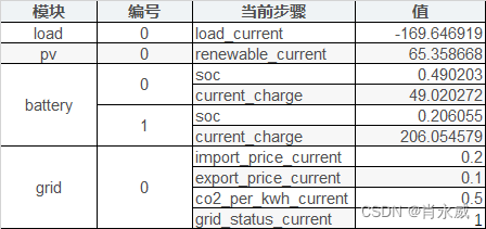
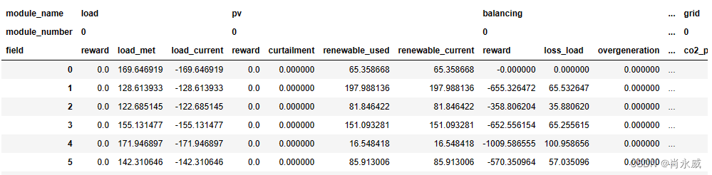
After passing control to the microgrid, the results can be viewed by viewing the logs of the microgrid or any module. There is one row for each operation in the microgrid log. Actions (such as the amount of load satisfied) and states (such as the current load) have values.

Note that the state value is the state value before the action was taken.

The columns are a pd.MultiIndex with three levels: module name, module name enum (e.g. the number of each module name we're in), and attributes. For example, since there is a load, all of its log entries will be available under the key("load", 0). Since there are two batteries, there will be both (battery, 0) and (battery, 1).

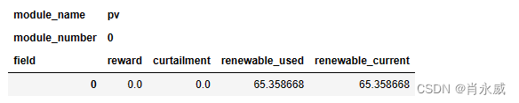
microgrid.log.loc[:, pd.IndexSlice['load', 0, :]]

microgrid.log.loc[:, pd.IndexSlice['pv', 0, :]]

microgrid.log.loc[:, 'battery']

3.4. Plotting the results

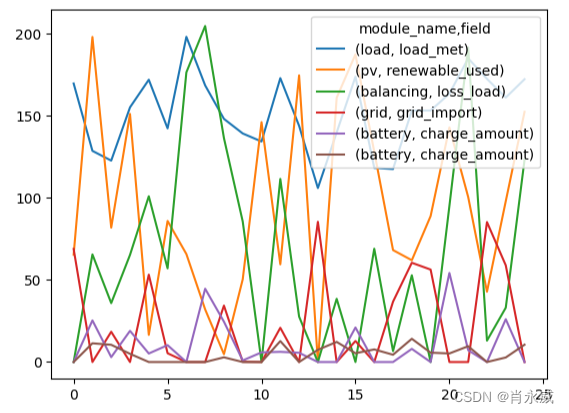
We can also take advantage of the pandas plotting functionality to view the results. To illustrate this, we will run the microgrid for another 24 steps with randomly sampled actions.

for _ in range(24):
    microgrid.run(microgrid.sample_action(strict_bound=True))

microgrid.log[[('load', 0, 'load_met'),
               ('pv', 0, 'renewable_used'),
               ('balancing', 0, 'loss_load'),
               ('grid', 0, 'grid_import'),
               ('battery',0,'charge_amount'),
               ('battery',1,'charge_amount')]].droplevel(axis=1, level=1).plot()

3.5. Microgrid log (data sheet)

microgrid.log

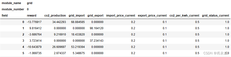
Expand to see the grid "grid" data:

microgrid.log[[('grid')]]

4. API Overview

4.1. Microgrid

Microgrid class for defining and simulating environments with various modules.

• method:

method name	illustrate
Microgrid.run(control[, normalized])	Run the microgrid step by step.
Microgrid.reset()	Reset microgrid and clear logs
Microgrid.sample_action([strict_bound, …])	Random actions are obtained within the action space of the microgrid.
Microgrid.get_log([as_frame, drop_singleton_key])	Collect control and response logs for the microgrid.
Microgrid.get_forecast_horizon()	Get the forecast bounds for the time series modules included in the microgrid.
Microgrid.get_empty_action([sample_flex_modules])	Operate the microgrid without setting a value.

• Serialization/IO/Conversion - Serialization/IO/Conversion:

name	illustrate
Microgrid.load(stream)	Load microgrid from yaml buffer.
Microgrid.dump([stream])	Save the microgrid to a YAML buffer.
Microgrid.from_nonmodular(nonmodular)	Converted from legacy legacy NonModularMicrogrid to Microgrid.
Microgrid.from_scenario([microgrid_number])	Load a pymgrid25 benchmark microgrid.
Microgrid.to_nonmodular()	Convert Microgrid to legacy NonModularMicrogrid.

4.2. Modules

pymgrid.modules.GridModule, a grid module.
By default, GridModule is a fixed module; it can be converted to a flex module via GridModule.as_flex. GridModule is the only built-in module that can be both fixed and flexible.

pymgrid.modules.RenewableModule, renewable energy module.
Classic examples of renewable energy are photovoltaics and wind turbines.

pymgrid.modules.BatteryModule, a battery module.
The battery module was fixed: you must pass battery control when calling Microgrid.run.

If you define a battery_transition_model, it must be YAML serializable if you plan to serialize your battery module or any microgrid containing batteries.
For example, you could define it as a class with a __call__ method and define yaml.YAMLObject as its metaclass. See the PyYAML documentation for details.

pymgrid.modules.GensetModule, generator set/genset module.
This module is a controllable source module; when used as a module in a microgrid, a generation production request must be sent to it.

pymgrid.modules.UnbalancedEnergyMod

4.3. Forecasting

Forecasting classes available for time series forecasting, and classes that allow users to define their own forecasters.

get_forecaster(), get the forecast function of the time series module.

4.4. Reinforcement Learning (RL) Environment

Environment classes for reinforcement learning using the OpenAI Gym API.

• Discrete

Environments with discrete action spaces.

DiscreteMicrogridEnv(modules[, …])

A discrete environment that implements priority lists as operations on a microgrid.

• Continuous

Environments with continuous action spaces.

ContinuousMicrogridEnv(modules[, …])

Microgrid environments with continuous action spaces.

4.5. Control algorithm

Control algorithms built into pymgrid, and references to external algorithms that can be deployed

• rule-based control

A heuristic algorithm for deploying modules via a priority list.

RuleBasedControl(microgrid[, priority_list, …])

Run rule-based (heuristic) control algorithms on the microgrid.

• Model Predictive Control

Algorithms that rely on future predictions and state transition models to determine optimal control.

ModelPredictiveControl(microgrid[, solver])

Run model predictive control algorithms on the microgrid.

• reinforcement learning

An algorithm that treats the microgrid as a Markov process and trains a black-box policy through repeated interactions with the environment. See subsequent articles for examples of using reinforcement learning to train such algorithms.

参考原文：
pymgrid documentation
Gonzague Henri (Total). pymgrid: An Open-Source Python Microgrid Simulator for Applied Artificial Intelligence Research (Papers Track). Neurips 2020