Coursera Wu Enda Neural Networks and Deep Learning Notes

Start Wu Enda deep learning spicy! !
Coursera DeepLearning
Netease Cloud Classroom Video

This deep learning has 5 courses, then the first course has 4 weeks:

---

Neural Networks and Deep Learning

Week 1

blow water

---

Week 2

2.1
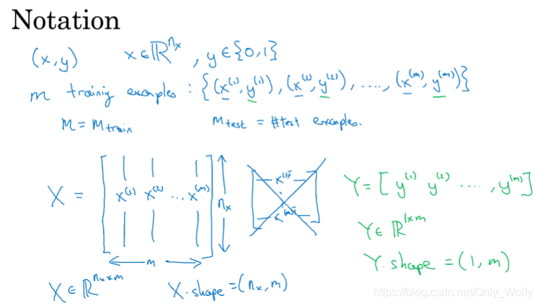
Let me talk about the definition of deep learning. In machine learning, each row of X seems to be a set of data, and here each column is a set of data.
Then n is the number of features, m is the number of samples, there are m_train, m_test, etc.:

2.2

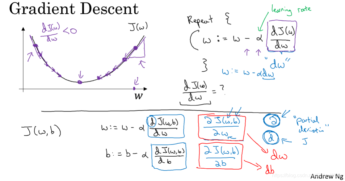
The familiar gradient descent, where J ( w , b ) can be written as dw for the partial derivative of w, and the same is true for the partial derivative of b.
Then if you want to find partial derivatives (there are multiple variables that take derivatives of a certain variable), use the d in the flower body, and the derivative is d.

Then here is not like machine learning, where w and b are fused into the θ matrix, w and b will be separated, w is a column vector, and b is a constant: 2.11 Use numpy's

dot
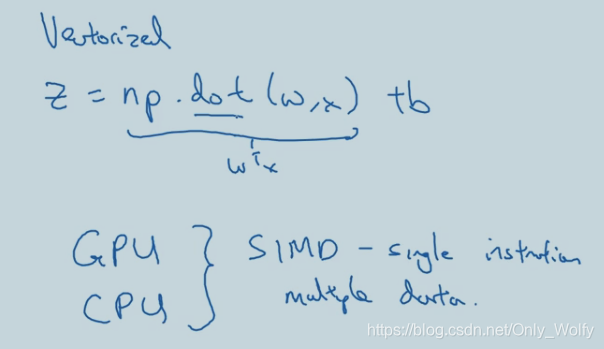
to do the dot product (.dot two vectors) And matrix multiplication (.dot two matrices or one vector and one matrix), note: dot product is different from matrix multiplication, dot product: a.*b, matrix multiplication: a*b if library function is called (not explicitly
used for loop), what kind of parallel operation will he do, and then it is related to SIMD, and then GPU is better at this SIMD operation than CPU (CPU is not bad), in short, library adjustment will be more efficient and concise than handwriting.
Put some introduction links:
np.dot() uses the method
vector inner product (dot product) and outer product (cross product) concept and geometric meaning

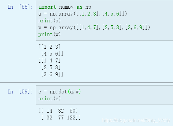
Test:

2.12
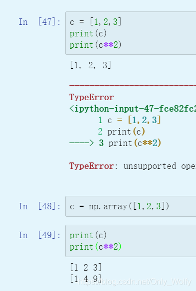
Then in order to improve efficiency, try not to use for loop explicitly, and Many functions can be called, for example, exp is to find a matrix that is the result of all the elements of the original matrix as the index of e (probably = = ): V**

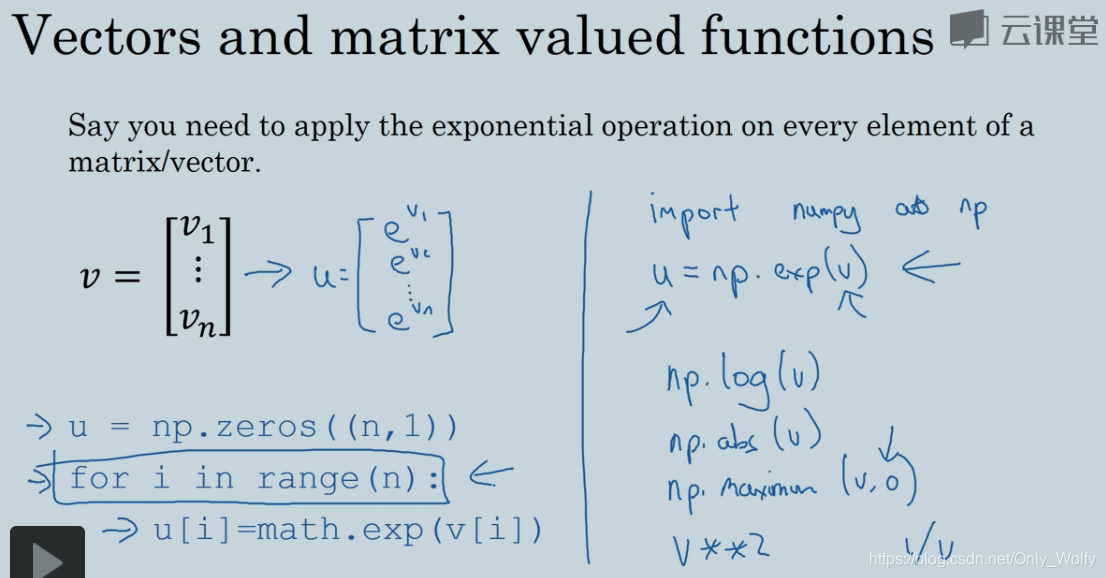
2 is the square of each element of the matrix:

2.13
here b should be 1 xm dimensional , but adding a constant to the matrix will add that element to each element, which is equivalent to matrix addition:

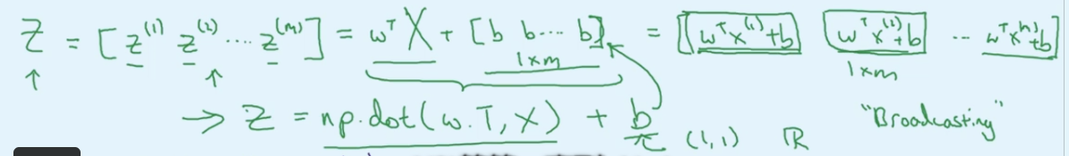
2.15 Broadcasting in Python
Remember some Python syntax

2.16 A note on python/numpy vectors

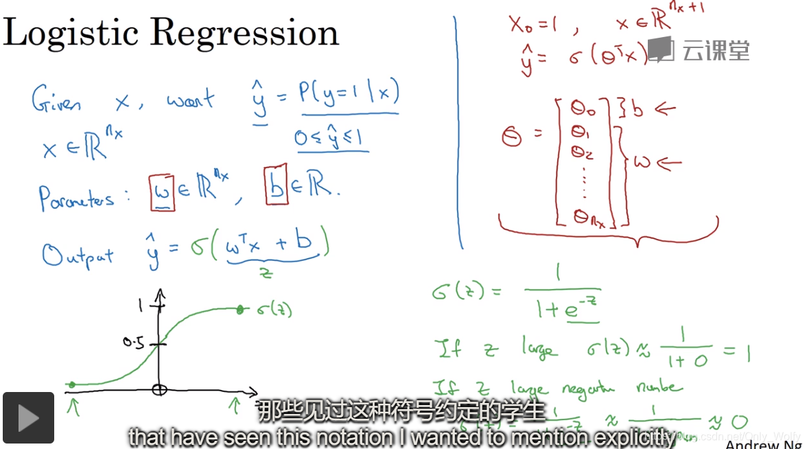
2.18 Explanation of logistic regression cost function (optional)
explains the derivation of logistic regression

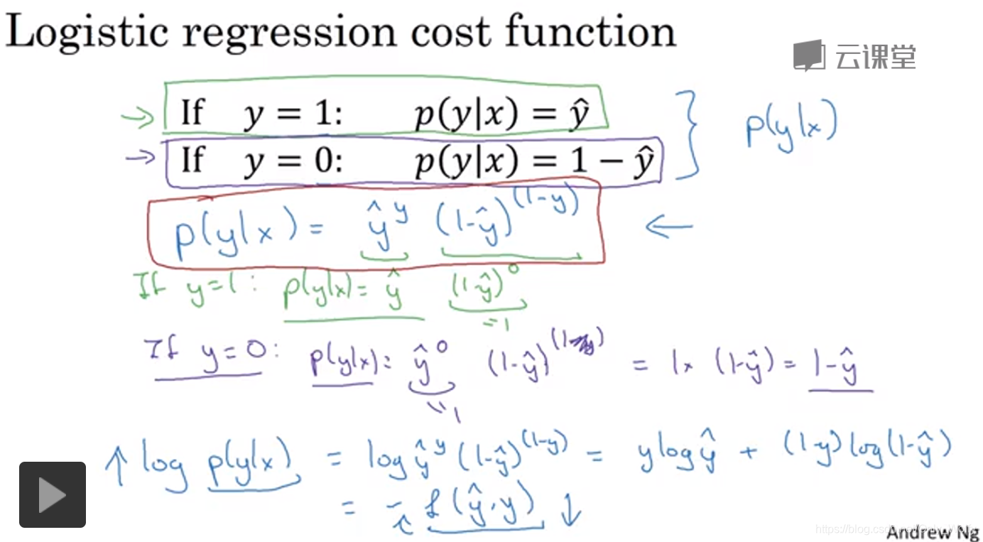
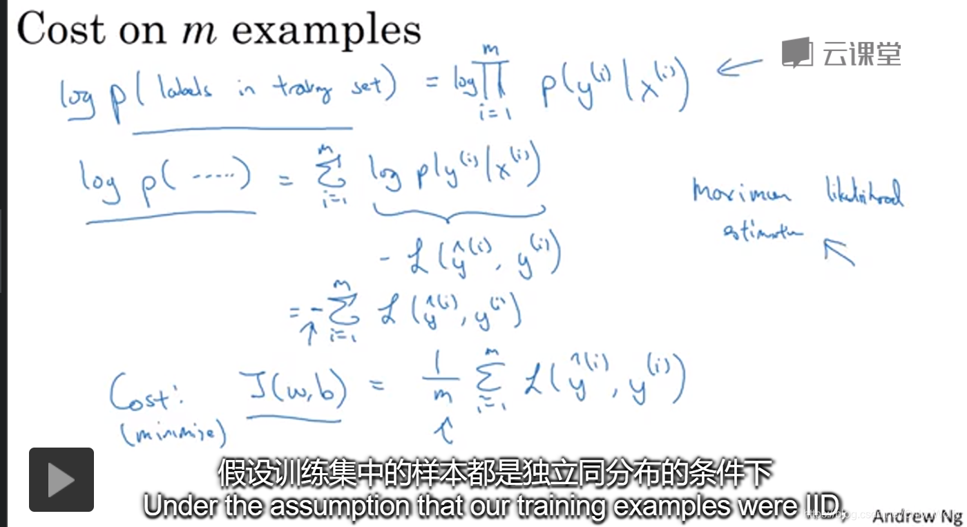
using the maximum likelihood estimation method, multiplying both sides by log:

Homework 1 Python Basics with numpy (optional)

Homework 2 Logistic Regression with a Neural Network mindset
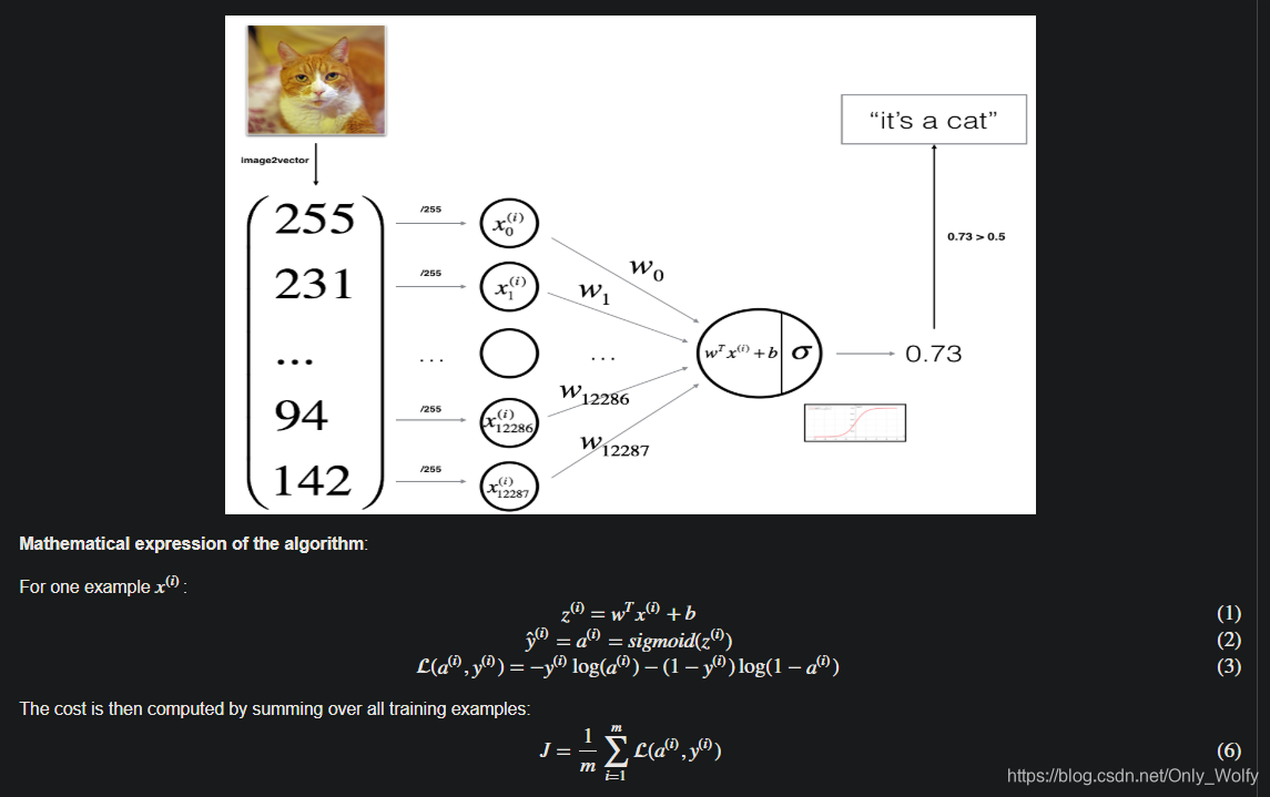
suddenly has an understanding of the L(a(i),y(i)) function: (L: the error of a certain sample, J: the overall average error)
if y (note and y_hat Distinguish) is 1, then roughly write it as: L = -ylog(a) = -log(a)
The larger a is, the more the algorithm thinks it should be 1, the larger log(a), and the smaller L is, The final statistics are J = 1/m sigma(L), the original intention is to minimize J, so the smaller the L, the better, and the bigger a, the better.
If y is 0, then it is: L = -(1-y )log(1-a) = - log(1-a), the smaller a is, the more the algorithm thinks it should be 0, the bigger 1-a is, the bigger log(1-a) is, then the smaller L is, then J The smaller is in line with the original intention of minimizing J.

pass. Here are the problems encountered:

1. There is a function that has three places to fill in, but I only filled in one to start the test, and then compile, but it says that the T of wT is not defined, I:? ? ? , If it weren't for someone next to me, I would start scolding. Then I searched for the error and couldn't find it, filled in the last two places, and the compilation passed...
2. Then here w, b wrote initialize_with_zeros(dim) at the beginning. . It was a coincidence, it was not written by the brain, and then I read the error and reported that the dimension was wrong, so I changed it to X_train.shape[1], and found that it was still wrong and changed it to [0]. Then shape[0] is because X.shape is (nx,m) nx refers to the number of elements in a set of samples, and m refers to the number of m sets of samples. So w is the 0th dimension.
   

Week 3

3.4 Vectorizing across multiple examples

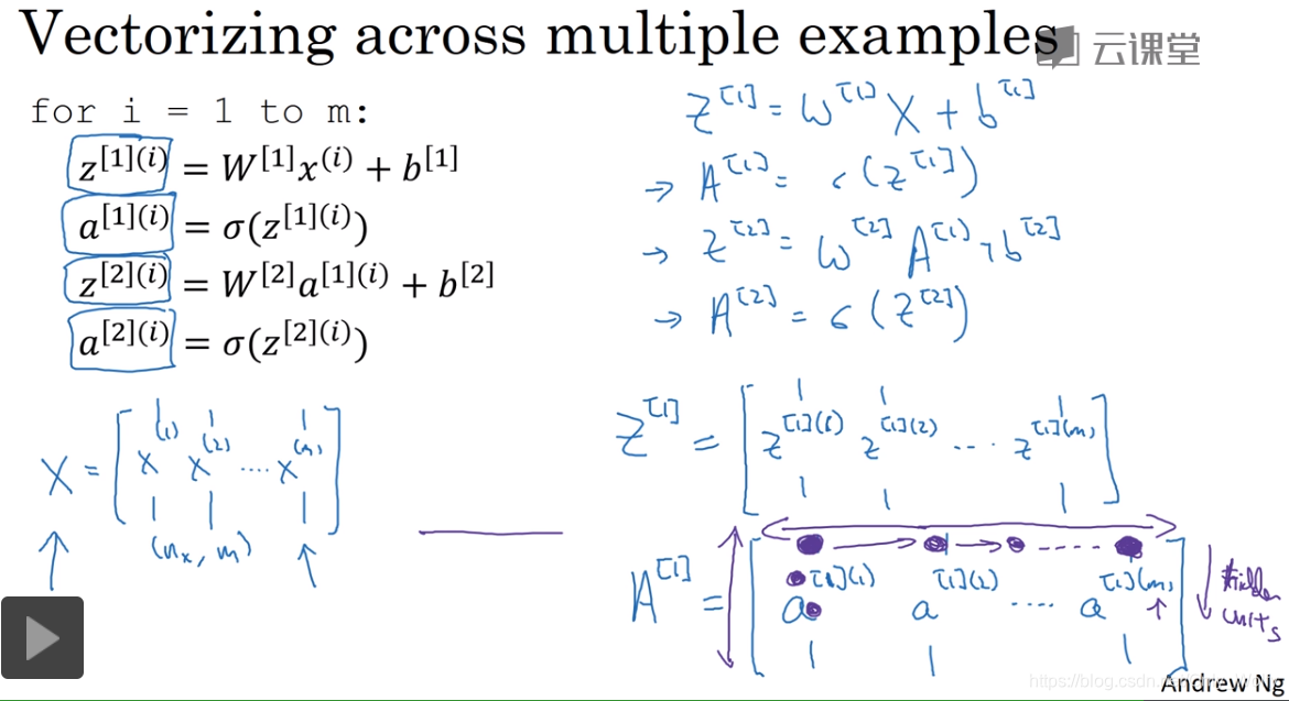
The brackets refer to the first layer, and the parentheses refer to the first sample (training sample).
Take the A array in the lower right corner as an example, the first row of the first column is the first point of the first layer of the neural network (of the first sample), the second row of the first column is the second point of the first layer, and the second column The first row is the first point of the first layer (of the second sample).
PS:$a_2^{[1]}$Indicates the second activation function a in the first hidden layer (that is, the circle in the second row of the first column circle)
3.5 Explanation for Vectorized Implementation


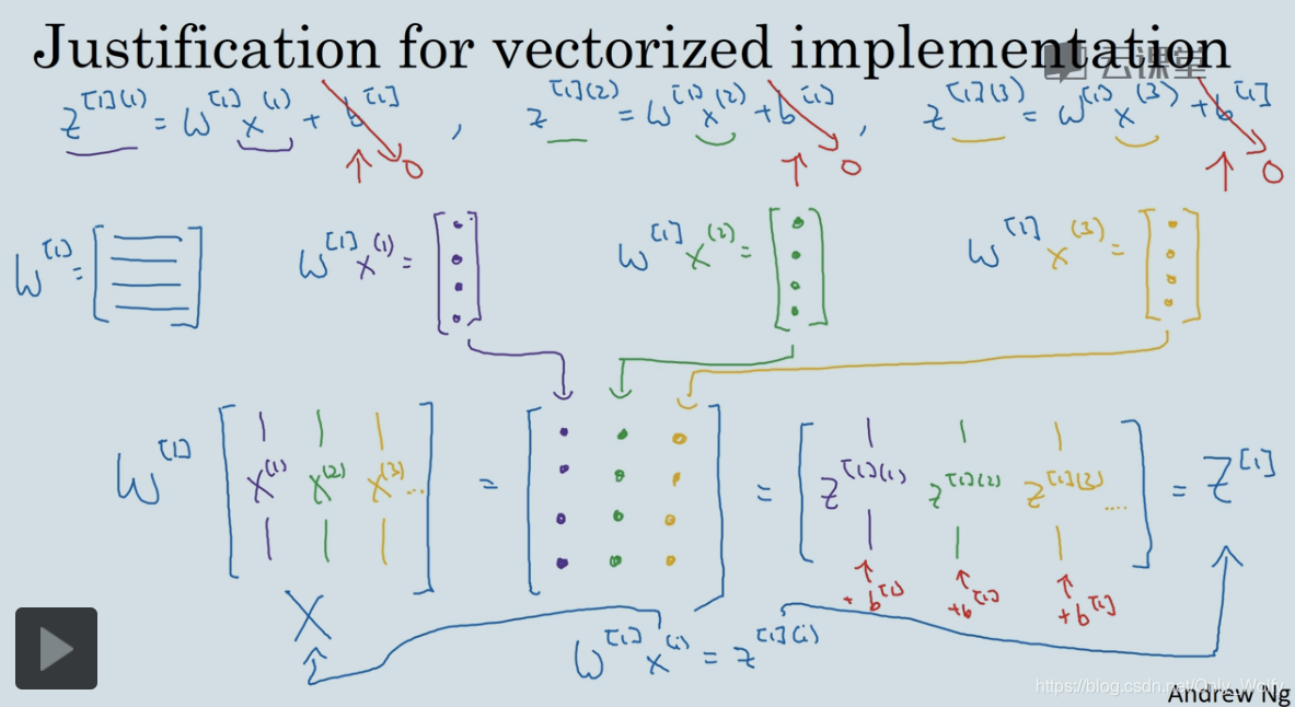
This section continues to talk about how to use vectorization, you can see w[1 ]x(1), w[1]x(2), w[1]x(3), are actually the values ​​of the first layer under different samples: z[1](1), z[1](2 ), z[1](3)... ...then arrange them in a row for the convenience of calculation. In the figure above, the code on the upper right and the code on the lower right have the same effect.

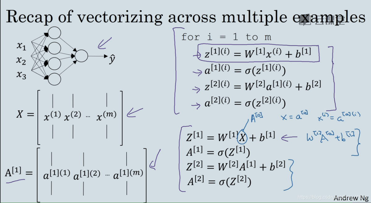
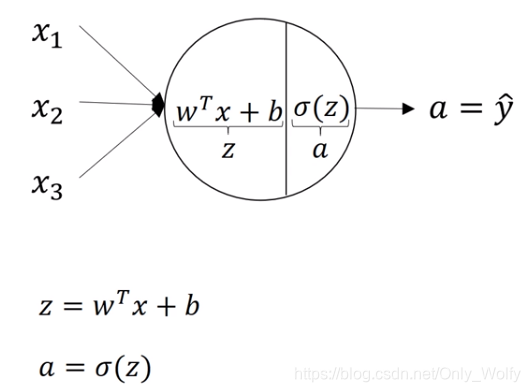
Finally, note that starting from the first layer of the hidden layer is [1], so the X matrix of the input layer can also be represented by A[0], Z refers to the input, which can be regarded as the left half of the ball, and A refers to the output It can be seen as the right half of the ball:

after knowing the code with only one hidden layer, multiple hidden layers just repeat the code.

3.6 Why do you need non-linear activation functions?

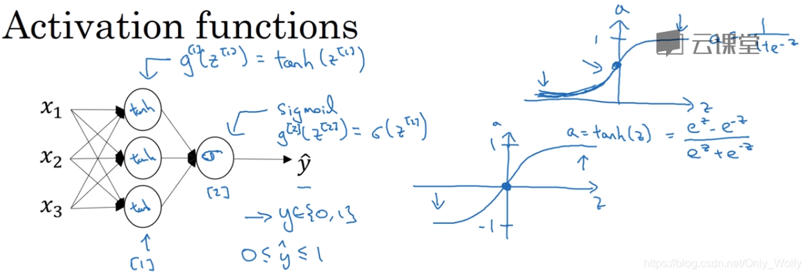
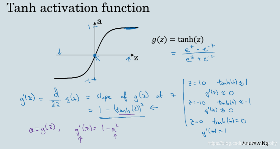
The activation function in this section uses sigmoid before the activation function ($a=\frac{1}{1+e^{-z}}$), but the tan function is used in the hidden layer ( $a=tanh\left(z\right)=\frac{e^z-e^{-z}}{e^z+e^{-z}}$), unless it is the output layer of binary classification , try not to use sigmoid, because:

At this time the value of the function is between 1 and -1 so the average value of the hidden layer activation function output will be closer to 0 Sometimes when you train a learning algorithm you may center your data and use tanh instead of Sigmiod Function to achieve the effect of data centering Data centering makes the average value of the data closer to zero

Wu Enda's original words... probably mean this.
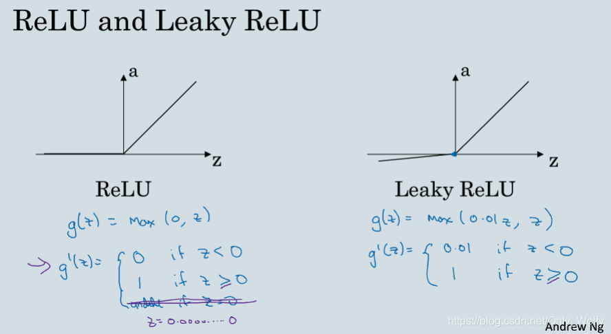
Then there is a ReLU function that is often used ( $a=max(0,z)$ ), then there is a Leaky ReLU (with leaky ReLU,$a=max(0.01z,z)$ ), relatively few people use 0.01z based on experience, and usually use ReLU.

In this lesson, I learned about popular and unpopular function selections. You need to choose according to your own topic/goal. You can run more on cross-data sets to see which one is better.

3.7 Why do you need non-linear activation functions?
The activation function is established to allow the neural network to achieve some interesting functions.

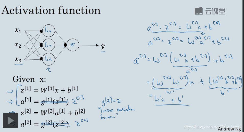
If there is no activation function (excluding the linear activation function ($g(z)=z$ )), then it is just like the a on the right, which islinear stacking, and then it is alsolinear, which has no practical significance, so a nonlinear activation function is required. The only linear activation function that needs to be used ($g(z)=z$ ) is the output of the last layer of the regression problem (ReLU can also be used here).

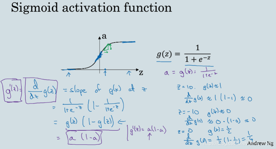
3.8 Derivatives of activation functions
introduces the derivative of the activation function



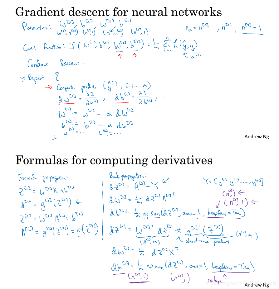
3.9 Gradient descent for Neural Networks
introduces how to perform gradient descent (derivation in the next section)

3.10 Backpropagation intuition (optional)

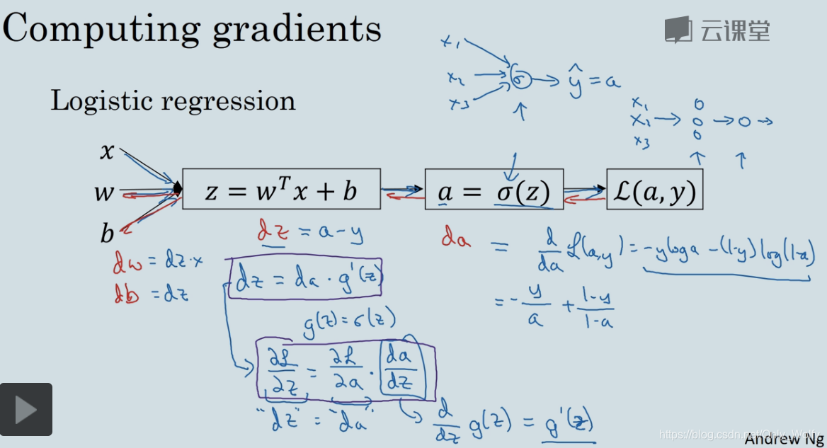
is derived using the chain rule, where the loss function is the cross entropy function :
$da=\frac{dL(a,y)}{da}$, how to get the derivation specifically, there are
$dz=\frac{dL}{da}\cdot \frac{d}{dz}=da\cdot p^{\prime }\left(z\right)$, the sigmoid function is used here (although hh is no longer used before)
$=da\cdot \sigma \left(z\right)\cdot (1-\sigma (z\left)\right)=da\cdot a\cdot (1-a)=a-y$
$dw=\frac{dL}{dz}\cdot \frac{dz}{dw}=dz\cdot x$
$db=\frac{dL}{dz}\cdot \frac{dz}{db}=Below\; dz$
is the formula derivation of the two hidden layers:

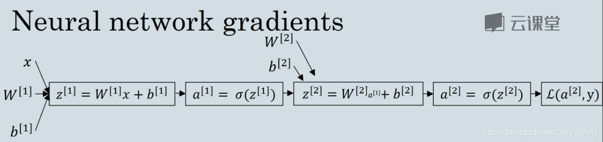
For the forward propagation of the 2 hidden layers (the left is the formula derivation, the right is the code)

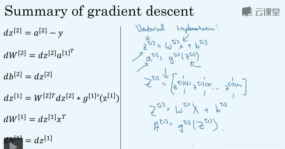
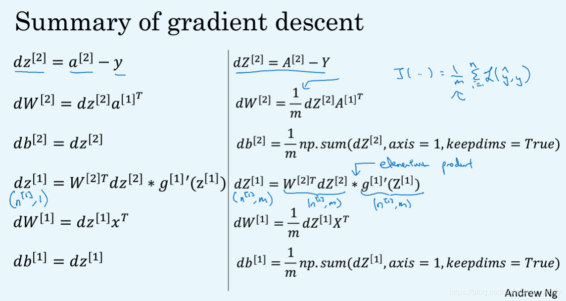
For the back propagation: (note that m is removed, because there are m groups)

the last point multiplication I don't quite understand why it is a dot product. ng said that it depends on the dimension, because two things of the same dimension are multiplied, so it is a dot product. (Huh?????) Think about it later, it should be the mathematical meaning inside, but it can be quickly distinguished by dimension (provided that the formula is listed correctly)

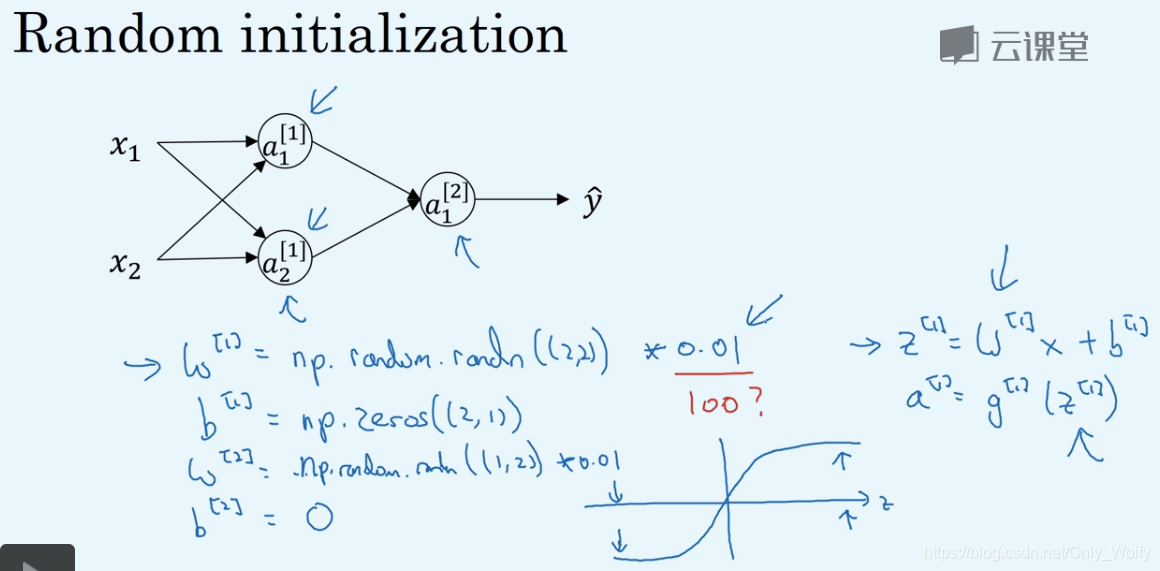
3.11 Random Initialization
If you put$w^{\left[1\right]}$ All initialized to 0, then the circles (hidden units) in the first column all calculate the same thing, no matter how many iterations, but we set up different hidden units to calculate different functions for them.

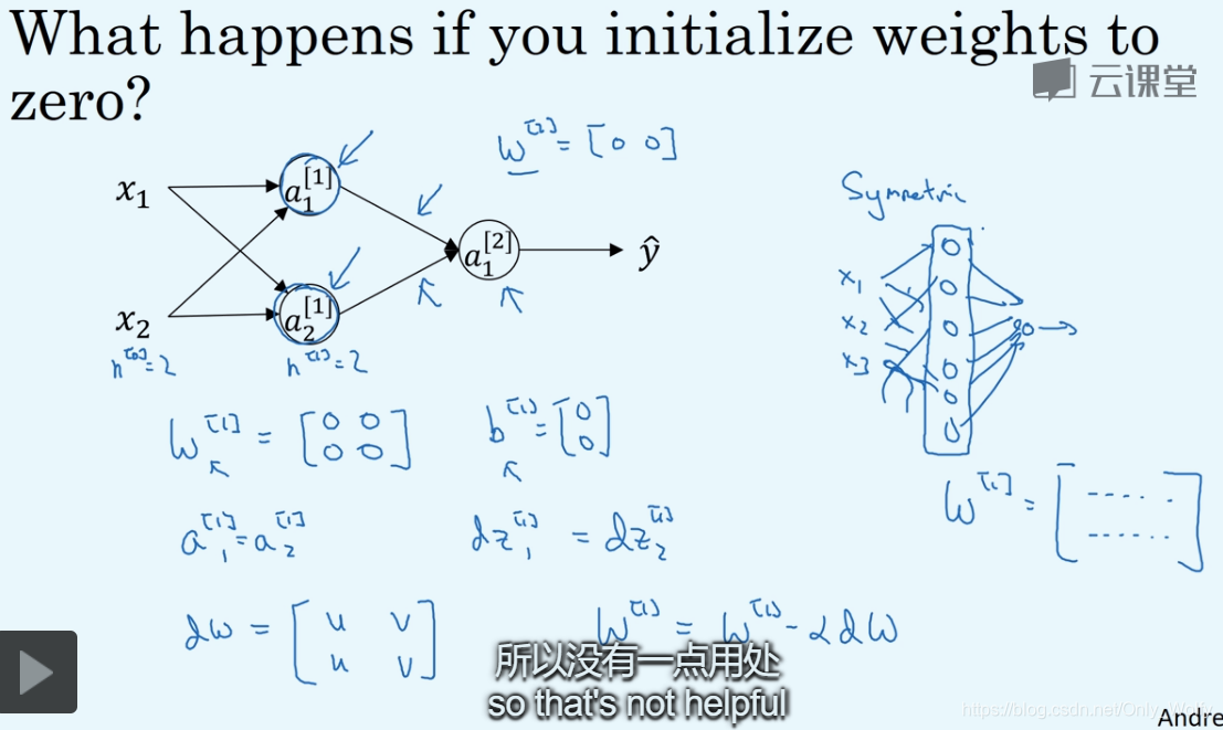
The solution is to randomize the array, and then take 0.01 instead of 100 because if the activation function is tanh or sigmoid, then the derivative will be small, which is not conducive to the subsequent gradient descent:

---

Week 4

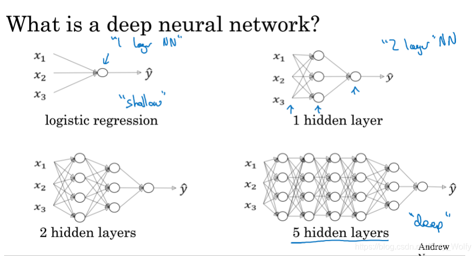
4.1 Deep L-layer neural network
has begun to build deep learning networks. Usually, a lot of layers are called deep, and then layer is the number of hidden layers + output layers.

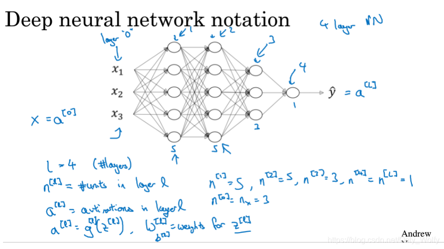
Here are the specifications of some symbols:
L refers to layer,$n^l$ is thellthThe number of nodes in layer$l$$a^l$ is the$The\; activation\; function\; of\; the\; l$ layer, namely$g^{[l]}(z^{\left[l\right]})$, so$a^{\left[0\right]}$ is$X$，$a^{\left[L\right]}$ That is$Yhat$ , predicted output,$W^{\left[l\right]}$ is the$L$ layer$W$，$b^{\left[l\right]}$ is the$l$ layer of$b$

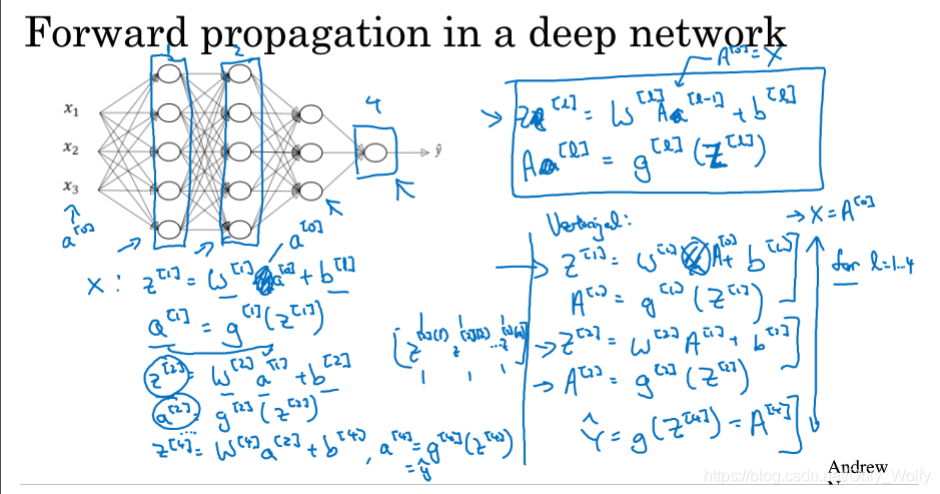
4.2 Forward Propagation in a Deep Network
forward pass formula. . Nothing is different, the only thing to pay attention to is to use for to loop$l$ , because there is no better way to speed up the calculation of each layer.

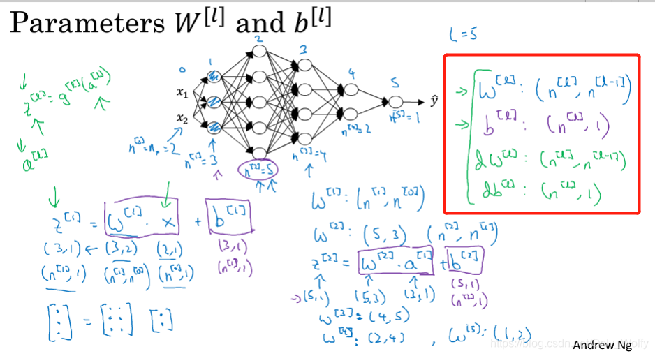
4.3 Getting your matrix dimensions right
This section talks about how to make your matrix dimensions correct:

• In the W matrix, because Z = WX + b, the number of rows of W is the number of rows of Z, and the number of columns is the number of rows of X.
  Then dW db is the same size as W and b respectively
• It is worth noting that because there are m samples for Z, A, and X, the number of columns must be changed from 1 to m (the letters of 1 sample are z, a, and x) 4.4 Why deep representations? Why use deep
  
  
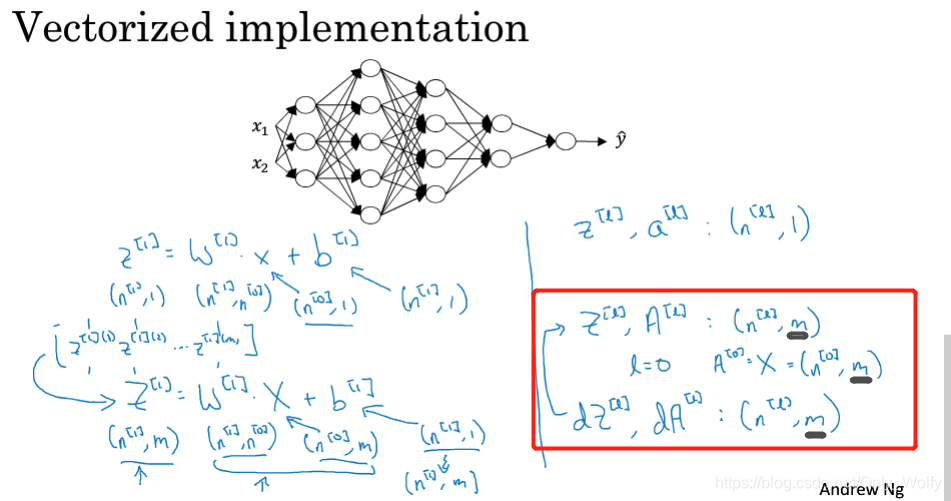
  learning
  ? / Why use more hidden layers for neural networks?
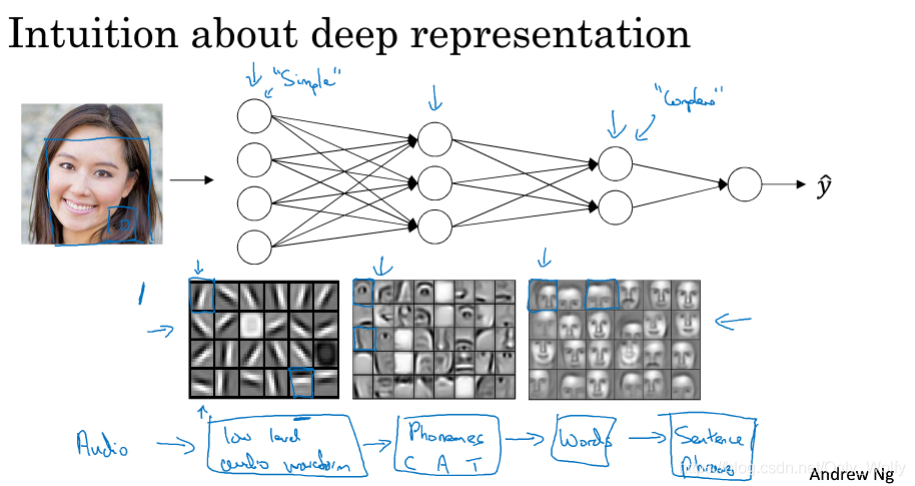
  The explanation here is that, taking face recognition as an example, the first layer is used to detect edges or relatively simple and rough features, the next layer detects some facial features, and then the third layer is the face.

  Some here feel that this is the operation of the brain, starting from the rough features, and then refining them step by step. I read some opinions before saying that the brain’s thinking is modeled after the neural network, but the human body does not have backpropagation, which means that the brain does not use backpropagation, but it still achieves the effect of the neural network.

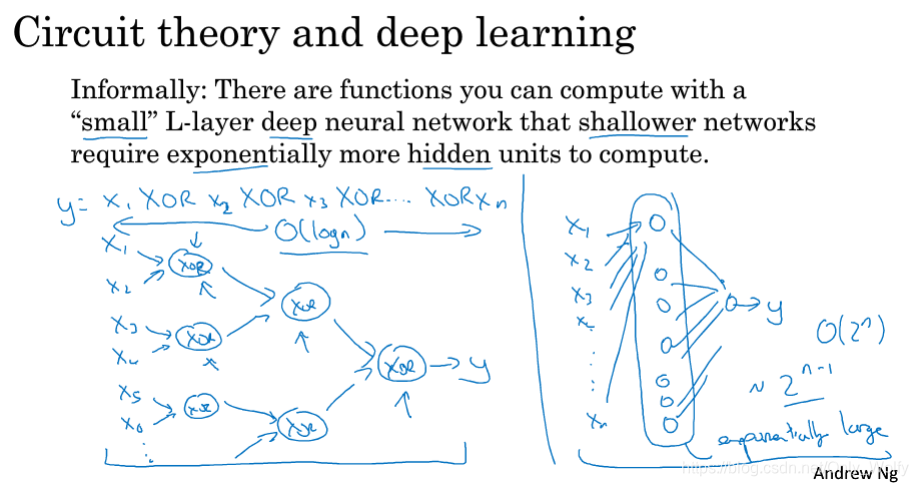
Another explanation is circuit theory. If there are n XORs, for the deep layer, just build a tree and use logn time to complete it. For a shallow layer, such as a hidden layer, 2^(n-1) points are needed (-1 is because n numbers have n-1 circles (XOR) to connect them), so the shallow layer needs time will increase exponentially.

Finally, in fact, when solving the problem at the beginning, it is recommended to start with logistic regression, and then increase the number of layers step by step if the effect is not good. Only certain problems require many layers.

4.5 Building blocks of deep neural networks
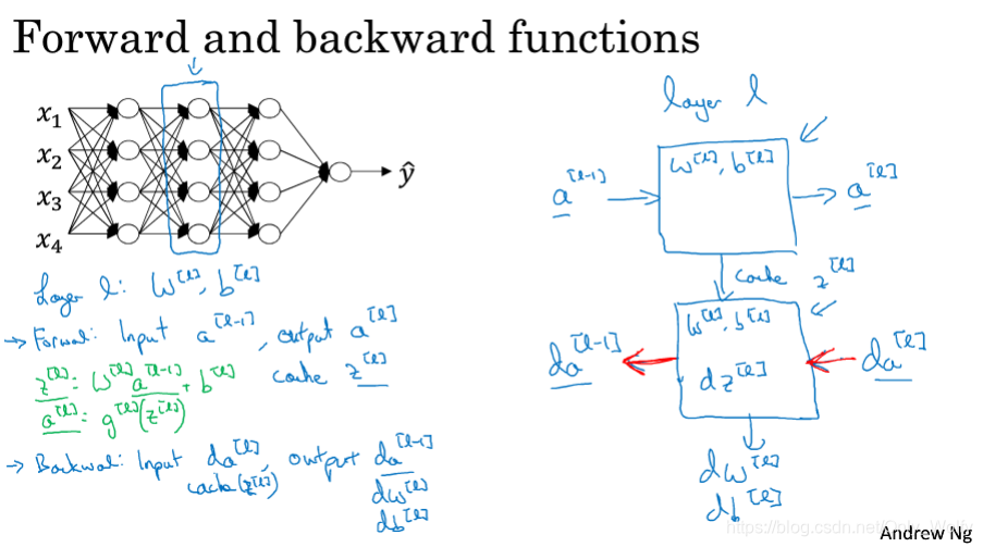
The following explains how to construct a deep neural network:are
on the left, and the general process is on the right. The blue (horizontal) arrow indicates the forward process, and the red reverse arrow indicates the backward process.

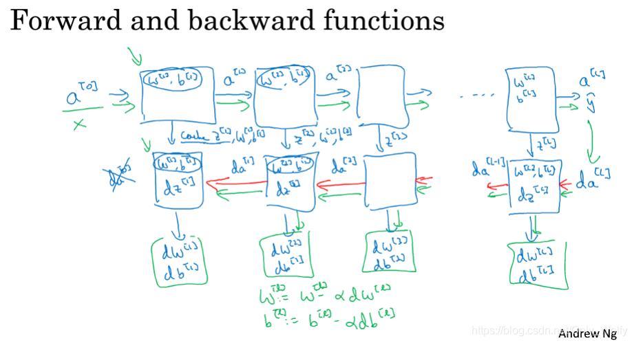
Detailed neural network forward and backward process, green indicates the process from beginning to end, blue is forward, red is backward, note that a cache will be recorded during forward, so that the parameters in the cache can be used conveniently during backward. Note that da[0] does not need to be calculated.

4.6 Forward and Backward Propagation
This section continues the content of the previous section, and then focuses on the bp formula. Here$d{a}^{[l-1]}$ I don't know how to get it. (Others who don’t understand can go back to 3.10 and below)
I understand, because there is$z^{[l]}=w^{[l]}{a}^{[l-1]}+b^{\left[l\right]}$，所以$\frac{dL}{d{a}^{[l-1]}}=\frac{dL}{d{z}^l}\cdot \frac{d{z}^l}{d{a}^{[l-1]}}=d{z}^l\cdot w^{\left[l\right]}$
Then the last line is$d{a}^{[l-1]}$ Substitute back to the first line:

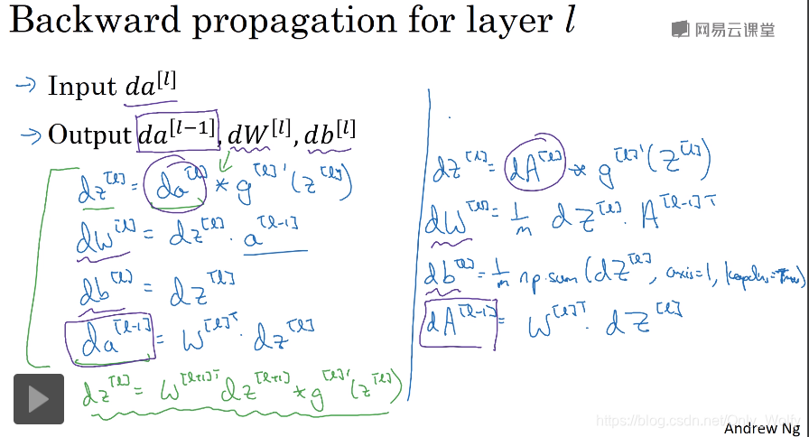
this$d{a}^{[l-1]}$代入$d{z}^{\left[l\right]}$ to get the green formula, which is the$d{z}^{\left[1\right]}$ Formula:

Summary: (This picture again) Remember to capitalize the letters, because there are m sets of data

One last point: I want to emphasize that if you think these formulas seem a bit abstract and difficult to understand, my suggestion is to do the homework carefully and then it will suddenly become clear. But I have to say that even now when I implement a machine learning algorithm, sometimes I'd also be amazed that my machine learning algorithms are proven to work because the complexity of machine learning comes from data rather than lines of code so sometimes you feel like you've written lines of code but aren't sure what they're doing and they end up producing Magical results because actually most of the magic isn't in the few lines of code you write, which may not be really that short, but it won't be thousands of lines of code that just happen to be typing in a lot of data even though I have been doing machine learning for many years and sometimes I am still surprised that my machine learning algorithm works because the complexity of the algorithm comes from the data and not necessarily the thousands of lines of code you write

The code of the neural network is usually not very long, but it can "work". The reason is not necessarily the code, but a large amount of data from quantitative changes to qualitative changes.

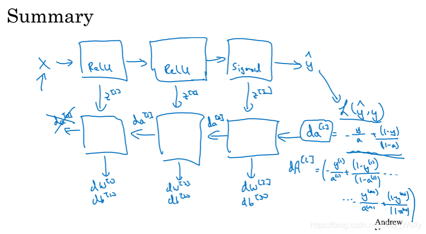
Finally, let's sort it out again : first get $d{a}^{\left[l\right]}$ (in the case of cross entropy is$\frac{-y}{a}+\frac{1-y}{1-a}$), then $d{z}^{\left[l\right]}、dw{\_}^{[l]}、d{b}^{\left[l\right]}$ , then by$d{z}^{\left[l\right]}$ yields$d{a}^{[l-1]}$ , so there are$d{z}^{[l-1]},d{w}^{[l-1]}、d{b}^{[l-1]}$ ……
(Figure of 3.10:)

4.7 Parameters vs Hyperparameters
Parameters vs hyperparameters:
what are hyperparameters? Hyperparameters are parameters that can control parameters, such as the number of iterations iter, the learning rate α, the number of hidden layers L, the number of hidden units in the hidden layer, and the selection of activation functions, which ultimately affect wlw^$w^l$ and$b^l$ , and future momentum (? momentum), minibatch size, regularization parameters, etc.

Selection of hyperparameters: You need to go through the circle on the left to continuously modify, such as the picture on the right, knowing that you have selected a satisfactory α. When starting a new project, you need to use this method to find the optimal hyperparameters. For familiar projects, you should also Check it every once in a while, because the optimal hyperparameters will change, because the CPU, GPU, network, and database are constantly being updated: Then

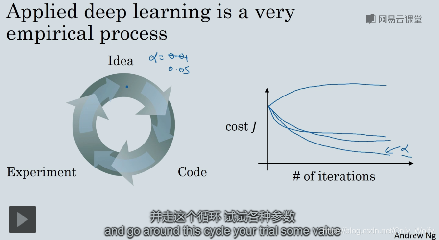
mention one of the unsatisfactory aspects of deep learning: you need to constantly try different hyperparameters The value of (then evaluate on the reserved cross-validation set or other sets, and select the optimal solution). In the second lesson, we provide some advice on how to systematically explore the hyperparameter space.

4.8 What does this have to do with the brain?
What is the similarity between deep learning and the brain? Answer: It doesn't matter.

What is the similarity between deep learning and the brain? I conclude that the similarities between them are not high. Let's first look at why people tend to compare deep learning with the human brain. When you build a neural network system, you use forward propagation and back propagation. Since it is difficult for us to intuitively explain why these complex equations can achieve ideal results, the analogy between deep learning and the human brain makes this process oversimplified, but it is easier to explain. The simplicity of this explanation makes it easier for the public to use various The media mentions, uses or reports about it and certainly sparks the public's imagination. There are indeed some parallels between this, such as logistic regression units and sigmoid activation functions. Here's an image of a brain neuron in this bio In the picture of a neuron in the sense, this neuron is actually a cell in your brain, and it will receive current signals from other neurons, such as neurons x1, x2, x3, or other neurons a1, a2,

course1 is over!