I saw a very interesting article today, which is related to medical image segmentation, but it is not like some previous work that blindly pursues high precision, because the medical field itself is a relatively special industry. For the model The accuracy requirements of the generated results are very high, which brings about a large number of parameters. The reason why I think this paper is very interesting is because the main point here is that it is ultra-lightweight but it does not lead to a significant drop in accuracy. .
The official paper address is here , as follows:

It can be seen that it has just been published.

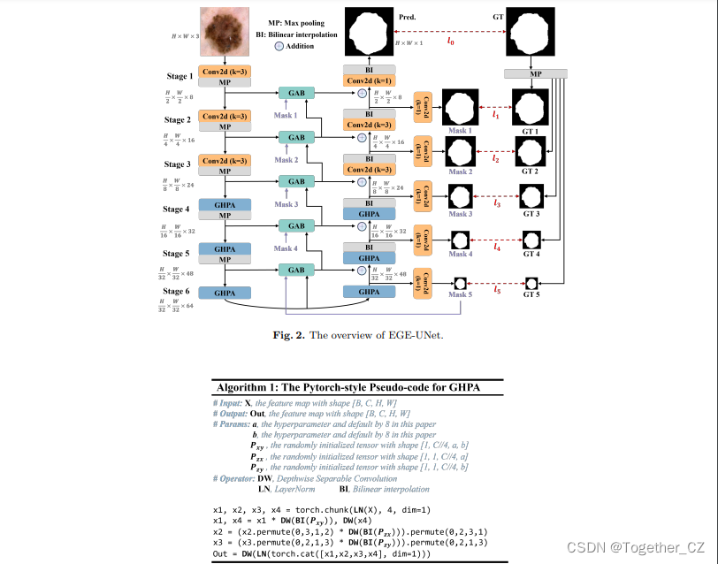
EGE-UNet combines two main modules:
Group multi-axis Hadamard Product Attention module (GHPA)
Group Aggregation Bridge module (GAB)
GHPA uses Hadamard Product Attention Mechanism (HPA) to classify different The HPA operation is performed on the axis to extract lesion information from multiple perspectives.
GAB fuses high-level semantic features and low-level detail features of different scales and the mask generated by the decoder through group aggregation, so as to effectively extract multi-scale information. By fusing the above two modules, the EGE-UNet model is proposed
. Excellent segmentation performance with very low complexity.
The design of EGE-UNet follows the U-shape architecture, including a symmetrical encoder-decoder part. The encoder consists of six stages, and the number of channels in each stage is {8, 16, 24, 32, 48, 64}. The first three stages employ ordinary convolutions, while the last three stages use the proposed GHPA to extract representation information from multiple views.
EGE-UNet integrates GAB at every stage between encoder and decoder. In addition, the model also utilizes deep supervision to generate mask predictions at different scales, which are used in the loss function as one of the inputs to GAB. Through the integration of these advanced modules, EGE-UNet significantly reduces parameters and computational load while improving segmentation performance over previous methods.
For further details, you can study the published papers yourself.
Here I also have a preliminary understanding, mainly because I want to actually use this ultra-lightweight network, because I think this type of network is more meaningful in real work, and the high-precision model with large parameters is of course very good. However, not all equipment in industrial or medical scenarios has such a high computing power that can support such a huge amount of calculations. If it can maintain good accuracy performance on a highly lightweight network basis, it is indeed very useful. practical.
The official open source project at the same time, the address is here , as follows:

I feel that the current number of stars is very small, and it is estimated that not many people know about it, so let me bring a wave of enthusiasm.
Judging from the readme, the practical training manual given by the author can be said to be extremely simple:

The data set is also ready, the address is here , as follows:

You can download it by yourself, the volume is not large, and it should be downloaded quickly.
Download Download and put it under the project data directory to decompress it, as shown below:

It can be seen that the author provides two sets of data sets at the same time, and the project source code uses the isic2017 data set by default.
Execute the train.py module directly on the terminal, as shown below:

The default iterative calculation of 300 epochs:

The screenshot of the training completion is as follows:

The results are stored in the results directory by default. As follows:

The trained model files are stored in the checkpoints directory, as follows:

The log directory stores the training log data, as shown below:

The output directory stores the actual test instance image visualization results, as shown below:

The official project only provides the code used for training and evaluation, and does not provide the code that can be used directly for offline reasoning, but based on the code of the training and evaluation part, you can develop the code for offline reasoning by yourself. Here I developed a dedicated one for easier use. The visual system interface, the example reasoning effect is as follows:

At this point, the basically complete practice is over. As mentioned earlier, the source code uses the isic2017 data set by default, so I will consider developing and training the model based on the isic2018 data set. You only need to modify the parameters in the configs directory. Yes, as follows:
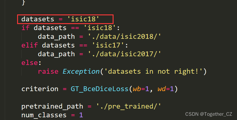
The modified config_setting module looks like this:
from torchvision import transforms
from utils import *

from datetime import datetime

class setting_config:
    """
    the config of training setting.
    """

    network = 'egeunet'
    model_config = {
        'num_classes': 1,
        'input_channels': 3,
        'c_list': [8,16,24,32,48,64],
        'bridge': True,
        'gt_ds': True,
    }

    datasets = 'isic18'
    if datasets == 'isic18':
        data_path = './data/isic2018/'
    elif datasets == 'isic17':
        data_path = './data/isic2017/'
    else:
        raise Exception('datasets in not right!')

    criterion = GT_BceDiceLoss(wb=1, wd=1)

    pretrained_path = './pre_trained/'
    num_classes = 1
    input_size_h = 256
    input_size_w = 256
    input_channels = 3
    distributed = False
    local_rank = -1
    num_workers = 0
    seed = 42
    world_size = None
    rank = None
    amp = False
    gpu_id = '0'
    batch_size = 8
    epochs = 300

    work_dir = 'results/' + network + '_' + datasets + '_' + datetime.now().strftime('%A_%d_%B_%Y_%Hh_%Mm_%Ss') + '/'

    print_interval = 20
    val_interval = 30
    save_interval = 100
    threshold = 0.5

    train_transformer = transforms.Compose([
        myNormalize(datasets, train=True),
        myToTensor(),
        myRandomHorizontalFlip(p=0.5),
        myRandomVerticalFlip(p=0.5),
        myRandomRotation(p=0.5, degree=[0, 360]),
        myResize(input_size_h, input_size_w)
    ])
    test_transformer = transforms.Compose([
        myNormalize(datasets, train=False),
        myToTensor(),
        myResize(input_size_h, input_size_w)
    ])

    opt = 'AdamW'
    assert opt in ['Adadelta', 'Adagrad', 'Adam', 'AdamW', 'Adamax', 'ASGD', 'RMSprop', 'Rprop', 'SGD'], 'Unsupported optimizer!'
    if opt == 'Adadelta':
        lr = 0.01 # default: 1.0 – coefficient that scale delta before it is applied to the parameters
        rho = 0.9 # default: 0.9 – coefficient used for computing a running average of squared gradients
        eps = 1e-6 # default: 1e-6 – term added to the denominator to improve numerical stability
        weight_decay = 0.05 # default: 0 – weight decay (L2 penalty)
    elif opt == 'Adagrad':
        lr = 0.01 # default: 0.01 – learning rate
        lr_decay = 0 # default: 0 – learning rate decay
        eps = 1e-10 # default: 1e-10 – term added to the denominator to improve numerical stability
        weight_decay = 0.05 # default: 0 – weight decay (L2 penalty)
    elif opt == 'Adam':
        lr = 0.001 # default: 1e-3 – learning rate
        betas = (0.9, 0.999) # default: (0.9, 0.999) – coefficients used for computing running averages of gradient and its square
        eps = 1e-8 # default: 1e-8 – term added to the denominator to improve numerical stability
        weight_decay = 0.0001 # default: 0 – weight decay (L2 penalty)
        amsgrad = False # default: False – whether to use the AMSGrad variant of this algorithm from the paper On the Convergence of Adam and Beyond
    elif opt == 'AdamW':
        lr = 0.001 # default: 1e-3 – learning rate
        betas = (0.9, 0.999) # default: (0.9, 0.999) – coefficients used for computing running averages of gradient and its square
        eps = 1e-8 # default: 1e-8 – term added to the denominator to improve numerical stability
        weight_decay = 1e-2 # default: 1e-2 – weight decay coefficient
        amsgrad = False # default: False – whether to use the AMSGrad variant of this algorithm from the paper On the Convergence of Adam and Beyond
    elif opt == 'Adamax':
        lr = 2e-3 # default: 2e-3 – learning rate
        betas = (0.9, 0.999) # default: (0.9, 0.999) – coefficients used for computing running averages of gradient and its square
        eps = 1e-8 # default: 1e-8 – term added to the denominator to improve numerical stability
        weight_decay = 0 # default: 0 – weight decay (L2 penalty)
    elif opt == 'ASGD':
        lr = 0.01 # default: 1e-2 – learning rate
        lambd = 1e-4 # default: 1e-4 – decay term
        alpha = 0.75 # default: 0.75 – power for eta update
        t0 = 1e6 # default: 1e6 – point at which to start averaging
        weight_decay = 0 # default: 0 – weight decay
    elif opt == 'RMSprop':
        lr = 1e-2 # default: 1e-2 – learning rate
        momentum = 0 # default: 0 – momentum factor
        alpha = 0.99 # default: 0.99 – smoothing constant
        eps = 1e-8 # default: 1e-8 – term added to the denominator to improve numerical stability
        centered = False # default: False – if True, compute the centered RMSProp, the gradient is normalized by an estimation of its variance
        weight_decay = 0 # default: 0 – weight decay (L2 penalty)
    elif opt == 'Rprop':
        lr = 1e-2 # default: 1e-2 – learning rate
        etas = (0.5, 1.2) # default: (0.5, 1.2) – pair of (etaminus, etaplis), that are multiplicative increase and decrease factors
        step_sizes = (1e-6, 50) # default: (1e-6, 50) – a pair of minimal and maximal allowed step sizes
    elif opt == 'SGD':
        lr = 0.01 # – learning rate
        momentum = 0.9 # default: 0 – momentum factor
        weight_decay = 0.05 # default: 0 – weight decay (L2 penalty)
        dampening = 0 # default: 0 – dampening for momentum
        nesterov = False # default: False – enables Nesterov momentum

    sch = 'CosineAnnealingLR'
    if sch == 'StepLR':
        step_size = epochs // 5 # – Period of learning rate decay.
        gamma = 0.5 # – Multiplicative factor of learning rate decay. Default: 0.1
        last_epoch = -1 # – The index of last epoch. Default: -1.
    elif sch == 'MultiStepLR':
        milestones = [60, 120, 150] # – List of epoch indices. Must be increasing.
        gamma = 0.1 # – Multiplicative factor of learning rate decay. Default: 0.1.
        last_epoch = -1 # – The index of last epoch. Default: -1.
    elif sch == 'ExponentialLR':
        gamma = 0.99 #  – Multiplicative factor of learning rate decay.
        last_epoch = -1 # – The index of last epoch. Default: -1.
    elif sch == 'CosineAnnealingLR':
        T_max = 50 # – Maximum number of iterations. Cosine function period.
        eta_min = 0.00001 # – Minimum learning rate. Default: 0.
        last_epoch = -1 # – The index of last epoch. Default: -1.
    elif sch == 'ReduceLROnPlateau':
        mode = 'min' # – One of min, max. In min mode, lr will be reduced when the quantity monitored has stopped decreasing; in max mode it will be reduced when the quantity monitored has stopped increasing. Default: ‘min’.
        factor = 0.1 # – Factor by which the learning rate will be reduced. new_lr = lr * factor. Default: 0.1.
        patience = 10 # – Number of epochs with no improvement after which learning rate will be reduced. For example, if patience = 2, then we will ignore the first 2 epochs with no improvement, and will only decrease the LR after the 3rd epoch if the loss still hasn’t improved then. Default: 10.
        threshold = 0.0001 # – Threshold for measuring the new optimum, to only focus on significant changes. Default: 1e-4.
        threshold_mode = 'rel' # – One of rel, abs. In rel mode, dynamic_threshold = best * ( 1 + threshold ) in ‘max’ mode or best * ( 1 - threshold ) in min mode. In abs mode, dynamic_threshold = best + threshold in max mode or best - threshold in min mode. Default: ‘rel’.
        cooldown = 0 # – Number of epochs to wait before resuming normal operation after lr has been reduced. Default: 0.
        min_lr = 0 # – A scalar or a list of scalars. A lower bound on the learning rate of all param groups or each group respectively. Default: 0.
        eps = 1e-08 # – Minimal decay applied to lr. If the difference between new and old lr is smaller than eps, the update is ignored. Default: 1e-8.
    elif sch == 'CosineAnnealingWarmRestarts':
        T_0 = 50 # – Number of iterations for the first restart.
        T_mult = 2 # – A factor increases T_{i} after a restart. Default: 1.
        eta_min = 1e-6 # – Minimum learning rate. Default: 0.
        last_epoch = -1 # – The index of last epoch. Default: -1.
    elif sch == 'WP_MultiStepLR':
        warm_up_epochs = 10
        gamma = 0.1
        milestones = [125, 225]
    elif sch == 'WP_CosineLR':
        warm_up_epochs = 20
The retraining startup log output looks like this:

The overall resource usage can be seen to be very low, as shown below:

Wait until the model training is completed and then look at the actual effect. If you are interested, you can try it yourself. Later, you can consider applying the ultra-lightweight model in this article to the actual project development process.