Move your little hand to make a fortune, give it a thumbs up!
A step-by-step guide to fine-tuning pretrained NLP models for any domain
Introduction
In today's world, the availability of pretrained NLP models greatly simplifies the interpretation of text data using deep learning techniques. However, while these models perform well on general tasks, they often lack domain-specific adaptability. This comprehensive guide [1] aims to walk you through the process of fine-tuning pretrained NLP models to improve domain-specific performance.
motivation
Although pretrained NLP models such as BERT and Universal Sentence Encoder (USE) can effectively capture the complexity of language, their performance in domain-specific applications may be limited due to the range of training datasets. This limitation becomes apparent when analyzing relationships within a particular domain.
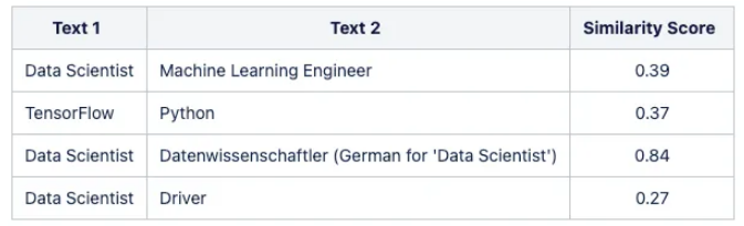
For example, when working with employment data, we want the model to recognize a closer relationship between the roles of "Data Scientist" and "Machine Learning Engineer", or a stronger association between "Python" and "TensorFlow". Unfortunately, general models often ignore these subtle relationships.
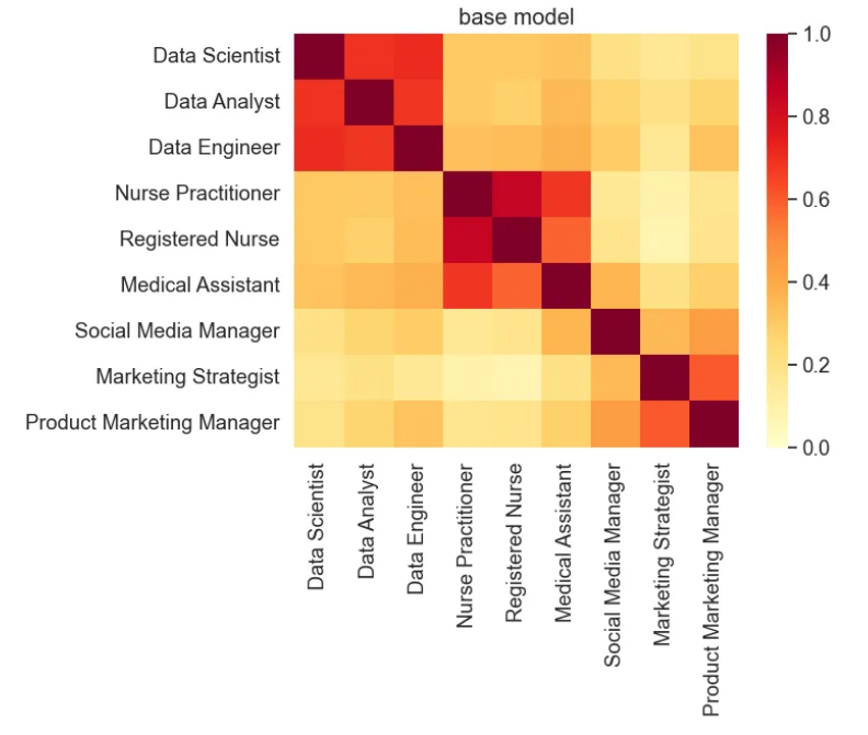
The following table shows the difference in similarity obtained from the basic multilingual USE model:
To solve this problem, we can use high-quality, domain-specific datasets to fine-tune pre-trained models. This adaptation process significantly enhances model performance and accuracy, unleashing the full potential of NLP models.
❝When dealing with large pretrained NLP models, it is recommended to deploy the base model first and consider fine-tuning only if its performance does not meet the specific problem at hand.
❞
This tutorial focuses on fine-tuning a Universal Sentence Encoder (USE) model using easily accessible open source data.
ML models can be fine-tuned through various strategies such as supervised learning and reinforcement learning. In this tutorial, we will focus on one-shot (few-shot) learning methods combined with Siamese architectures for the fine-tuning process.
theoretical framework
ML models can be fine-tuned through various strategies such as supervised learning and reinforcement learning. In this tutorial, we will focus on one-shot (few-shot) learning methods combined with Siamese architectures for the fine-tuning process.
method
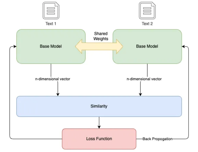
In this tutorial, we use a Siamese neural network, which is a specific type of artificial neural network. The network utilizes shared weights to simultaneously process two different input vectors to compute comparable output vectors. Inspired by one-shot learning, this approach has been shown to be particularly effective at capturing semantic similarity, although it may require longer training time and lacks a probabilistic output.
Siamese neural networks create an "embedding space" in which related concepts are closely located, enabling the model to better discern semantic relationships.
-
双分支和共享权重:该架构由两个相同的分支组成,每个分支都包含一个具有共享权重的嵌入层。这些双分支同时处理两个输入,无论是相似的还是不相似的。 -
相似性和转换:使用预先训练的 NLP 模型将输入转换为向量嵌入。然后该架构计算向量之间的相似度。相似度得分(范围在 -1 到 1 之间)量化两个向量之间的角距离,作为它们语义相似度的度量。 -
对比损失和学习:模型的学习以“对比损失”为指导,即预期输出(训练数据的相似度得分)与计算出的相似度之间的差异。这种损失指导模型权重的调整,以最大限度地减少损失并提高学习嵌入的质量。
数据概览
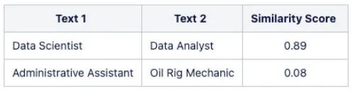
为了使用此方法对预训练的 NLP 模型进行微调,训练数据应由文本字符串对组成,并附有它们之间的相似度分数。
训练数据遵循如下所示的格式:
在本教程中,我们使用源自 ESCO 分类数据集的数据集,该数据集已转换为基于不同数据元素之间的关系生成相似性分数。
❝准备训练数据是微调过程中的关键步骤。假设您有权访问所需的数据以及将其转换为指定格式的方法。由于本文的重点是演示微调过程,因此我们将省略如何使用 ESCO 数据集生成数据的详细信息。
ESCO 数据集可供开发人员自由使用,作为各种应用程序的基础,这些应用程序提供自动完成、建议系统、职位搜索算法和职位匹配算法等服务。本教程中使用的数据集已被转换并作为示例提供,允许不受限制地用于任何目的。
❞
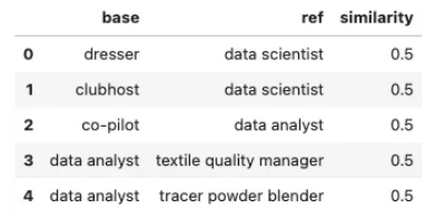
让我们首先检查训练数据:
import pandas as pd

# Read the CSV file into a pandas DataFrame
data = pd.read_csv("./data/training_data.csv")

# Print head
data.head()
起点:基线模型
首先,我们建立多语言通用句子编码器作为我们的基线模型。在进行微调过程之前,必须设置此基线。
在本教程中,我们将使用 STS 基准和相似性可视化示例作为指标来评估通过微调过程实现的更改和改进。
❝STS 基准数据集由英语句子对组成,每个句子对都与相似度得分相关联。在模型训练过程中,我们评估模型在此基准集上的性能。每次训练运行的持久分数是数据集中预测相似性分数和实际相似性分数之间的皮尔逊相关性。
These scores ensure that when the model is fine-tuned on our context-specific training data, it retains some level of generalizability.
❞
# Loads the Universal Sentence Encoder Multilingual module from TensorFlow Hub.
base_model_url = "https://tfhub.dev/google/universal-sentence-encoder-multilingual/3"
base_model = tf.keras.Sequential([
    hub.KerasLayer(base_model_url,
                   input_shape=[],
                   dtype=tf.string,
                   trainable=False)
])

# Defines a list of test sentences. These sentences represent various job titles.
test_text = ['Data Scientist', 'Data Analyst', 'Data Engineer',
             'Nurse Practitioner', 'Registered Nurse', 'Medical Assistant',
             'Social Media Manager', 'Marketing Strategist', 'Product Marketing Manager']

# Creates embeddings for the sentences in the test_text list.
# The np.array() function is used to convert the result into a numpy array.
# The .tolist() function is used to convert the numpy array into a list, which might be easier to work with.
vectors = np.array(base_model.predict(test_text)).tolist()

# Calls the plot_similarity function to create a similarity plot.
plot_similarity(test_text, vectors, 90, "base model")

# Computes STS benchmark score for the base model
pearsonr = sts_benchmark(base_model)
print("STS Benachmark: " + str(pearsonr))
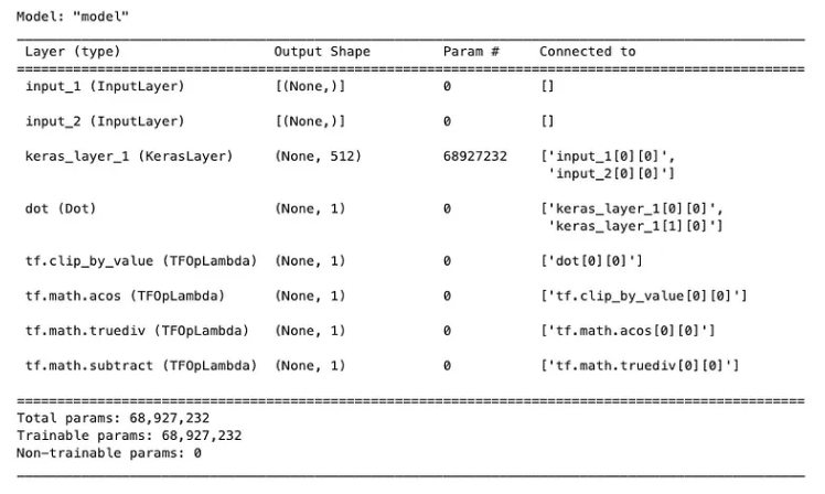
Fine-tuning the model
The next step involves building a Siamese model architecture using the baseline model and fine-tuning it using our domain-specific data.
# Load the pre-trained word embedding model
embedding_layer = hub.load(base_model_url)

# Create a Keras layer from the loaded embedding model
shared_embedding_layer = hub.KerasLayer(embedding_layer, trainable=True)

# Define the inputs to the model
left_input = keras.Input(shape=(), dtype=tf.string)
right_input = keras.Input(shape=(), dtype=tf.string)

# Pass the inputs through the shared embedding layer
embedding_left_output = shared_embedding_layer(left_input)
embedding_right_output = shared_embedding_layer(right_input)

# Compute the cosine similarity between the embedding vectors
cosine_similarity = tf.keras.layers.Dot(axes=-1, normalize=True)(
    [embedding_left_output, embedding_right_output]
)

# Convert the cosine similarity to angular distance
pi = tf.constant(math.pi, dtype=tf.float32)
clip_cosine_similarities = tf.clip_by_value(
    cosine_similarity, -0.99999, 0.99999
)
acos_distance = 1.0 - (tf.acos(clip_cosine_similarities) / pi)

# Package the model
encoder = tf.keras.Model([left_input, right_input], acos_distance)

# Compile the model
encoder.compile(
    optimizer=tf.keras.optimizers.Adam(
        learning_rate=0.00001,
        beta_1=0.9,
        beta_2=0.9999,
        epsilon=0.0000001,
        amsgrad=False,
        clipnorm=1.0,
        name="Adam",
    ),
    loss=tf.keras.losses.MeanSquaredError(
        reduction=keras.losses.Reduction.AUTO, name="mean_squared_error"
    ),
    metrics=[
        tf.keras.metrics.MeanAbsoluteError(),
        tf.keras.metrics.MeanAbsolutePercentageError(),
    ],
)

# Print the model summary
encoder.summary()
-
Fit model
# Define early stopping callback
early_stop = keras.callbacks.EarlyStopping(
    monitor="loss", patience=3, min_delta=0.001
)

# Define TensorBoard callback
logdir = os.path.join(".", "logs/fit/" + datetime.now().strftime("%Y%m%d-%H%M%S"))
tensorboard_callback = keras.callbacks.TensorBoard(log_dir=logdir)

# Model Input
left_inputs, right_inputs, similarity = process_model_input(data)

# Train the encoder model
history = encoder.fit(
    [left_inputs, right_inputs],
    similarity,
    batch_size=8,
    epochs=20,
    validation_split=0.2,
    callbacks=[early_stop, tensorboard_callback],
)

# Define model input
inputs = keras.Input(shape=[], dtype=tf.string)

# Pass the input through the embedding layer
embedding = hub.KerasLayer(embedding_layer)(inputs)

# Create the tuned model
tuned_model = keras.Model(inputs=inputs, outputs=embedding)
evaluation result
Now that we have the fine-tuned model, let's re-evaluate it and compare the results to those of the base model.
# Creates embeddings for the sentences in the test_text list.
# The np.array() function is used to convert the result into a numpy array.
# The .tolist() function is used to convert the numpy array into a list, which might be easier to work with.
vectors = np.array(tuned_model.predict(test_text)).tolist()

# Calls the plot_similarity function to create a similarity plot.
plot_similarity(test_text, vectors, 90, "tuned model")

# Computes STS benchmark score for the tuned model
pearsonr = sts_benchmark(tuned_model)
print("STS Benachmark: " + str(pearsonr))
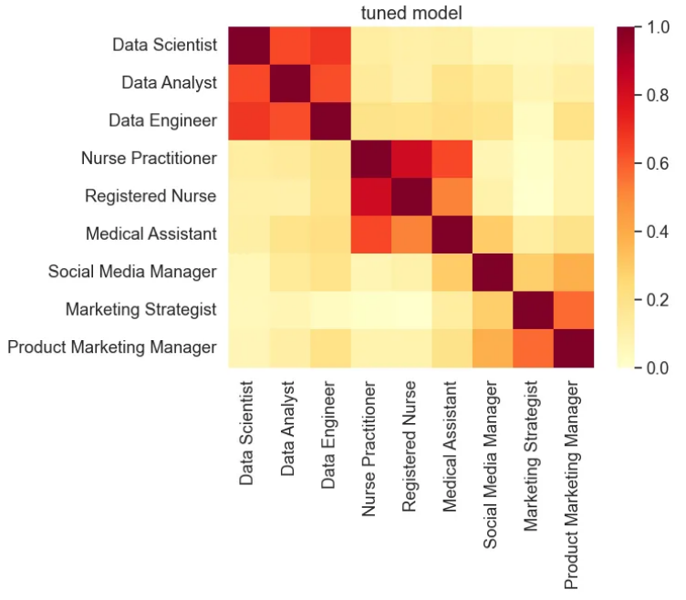
Based on fine-tuning the model on a relatively small dataset, the STS benchmark scores are comparable to those of the baseline model, indicating that the tuned model is still generalizable. However, the similarity visualization shows that the similarity score between similar titles is enhanced, while that of dissimilar titles is decreased.
Summarize
Fine-tuning a pretrained NLP model for domain adaptation is a powerful technique that can improve its performance and accuracy in specific contexts. By leveraging high-quality, domain-specific datasets and Siamese neural networks, we can enhance the model's ability to capture semantic similarity.
This tutorial provides a step-by-step guide to the fine-tuning process, using the Universal Sentence Encoder (USE) model as an example. We explore the theoretical framework, data preparation, baseline model evaluation and practical fine-tuning process. The results demonstrate the effectiveness of fine-tuning in enhancing the in-domain similarity score.
By following this approach and adapting it to your specific domain, you can unlock the full potential of pretrained NLP models and achieve better results in natural language processing tasks
Reference
Source: https://towardsdatascience.com/domain-adaption-fine-tune-pre-trained-nlp-models-a06659ca6668
This article is published by mdnice multi-platform