Introductory Guide to Deep Learning in 2023 (9) - SIMD and General GPU Programming
Deep learning has had an indissoluble bond with GPU from the very beginning, because computing power is an integral part of deep learning.
Today, although multi-tasking programming has been deeply rooted in the hearts of the people, many students have not been exposed to SIMD instructions on the CPU, let alone GPGPU programming. In this article, we will first scan SIMD and GPU programming, so that everyone can have a perceptual understanding when they use it in the future.
cpu world
Let's start with multithreading
Previous programming languages did not support multithreading, and required operating systems and libraries to provide multithreading capabilities, such as the pthread library. Today, there are still platforms that do not support multi-threading by default, such as wasm.
The Java language, which came out in 1995, has supported multithreading since version 1.0, although there was no major improvement in multithreading until version 5.0. The C++ language has supported multithreading since C++11.
Let's look at an example of using C++ multithreading to implement matrix multiplication:
#include <mutex>
    #include <thread>

        // 矩阵维度
        const int width = 4;

        // 矩阵
        int A[width][width] = {


            {

    1, 2, 3, 4},
            {

    5, 6, 7, 8},
            {

    9, 10, 11, 12},
            {

    13, 14, 15, 16}
        };
        int B[width][width] = {


            {

    1, 0, 0, 0},
            {

    0, 1, 0, 0},
            {

    0, 0, 1, 0},
            {

    0, 0, 0, 1}
        };
        int C[width][width] = {

    0};

        // 互斥锁
        std::mutex mtx;

        // 计算线程
        void calculate(int row) {


            for (int col = 0; col < width; col++) {


                if (row < width && col < width) {


                    mtx.lock();
                    C[row][col] = A[row][col] + B[row][col];
                    mtx.unlock();
                }
            }
        }

        int main() {


            // 创建线程
            std::thread t1(calculate, 0);
            std::thread t2(calculate, 1);
            std::thread t3(calculate, 2);
            std::thread t4(calculate, 3);

            // 等待线程结束
            t1.join();
            t2.join();
            t3.join();
            t4.join();

            // 打印结果
            for (int i = 0; i < width; i++) {


                for (int j = 0; j < width; j++) {


                    printf("%d ", C[i][j]);
                }
                printf("\n");
            }
        }
We give it a CMakeLists.txt:
cmake_minimum_required(VERSION 3.10)

# Set the project name
project(MatrixAddO)

# Set the C++ standard
set(CMAKE_CXX_STANDARD 11)
set(CMAKE_CXX_STANDARD_REQUIRED True)

# Add the executable
add_executable(matrix_add matadd.cpp)
Everyone should be familiar with this code, so I won't explain it much. It is now standard to support C++11 and above.
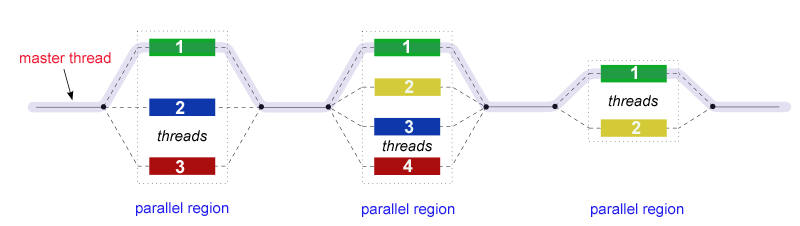
OpenMP
Long before threads were written into the C++11 standard, there were many frameworks for concurrent programming, such as MPI and OpenMP.
OpenMP is a multi-threaded concurrent programming API that supports cross-platform shared memory. It uses C, C++ and Fortran languages and can run on a variety of processor systems and operating systems. It is led by the OpenMP Architecture Review Board (ARB), and is jointly defined and managed by a number of computer hardware and software vendors.
OpenMP was first released in 1997, when it only supported the Fortran language. In 1998, C/C++ was supported.
Let's take a look at how to use OpenMP to implement concurrent calculations of matrices:
#include <iostream>
#include <omp.h>
#include <vector>

std::vector<std::vector<int>>
matrixAdd(const std::vector<std::vector<int>> &A,
          const std::vector<std::vector<int>> &B) {


  int rows = A.size();
  int cols = A[0].size();

  std::vector<std::vector<int>> C(rows, std::vector<int>(cols));

#pragma omp parallel for collapse(2)
  for (int i = 0; i < rows; i++) {


    for (int j = 0; j < cols; j++) {


      C[i][j] = A[i][j] + B[i][j];
    }
  }

  return C;
}

int main() {


  std::vector<std::vector<int>> A = {

    {

    1, 2, 3}, {

    4, 5, 6}, {

    7, 8, 9}};

  std::vector<std::vector<int>> B = {

    {

    9, 8, 7}, {

    6, 5, 4}, {

    3, 2, 1}};

  std::vector<std::vector<int>> C = matrixAdd(A, B);

  for (const auto &row : C) {


    for (int val : row) {


      std::cout << val << " ";
    }
    std::cout << std::endl;
  }

  return 0;
}
#pragma omp parallel for collapse(2)is an OpenMP pragma used to denote a parallel region in which nested loops are to be executed in parallel. Let's explain the various parts of this directive in detail:
#pragma omp: This is a compilation directive, indicating that the following code will be parallelized using OpenMP.
parallel for: This is a combination instruction, indicating that the following for loop will be executed in parallel on multiple threads. Each thread will process a portion of the loop, speeding up the execution of the entire loop.
collapse(2): This is an optional clause to indicate parallelization of nested loops. In this example, collapse(2) means to merge the two nested loops (i.e. the outer and inner loops) into a single parallel loop. This allows better utilization of the performance of multi-core processors due to the increased parallelism.
In our matrix addition example, #pragma omp parallel for collapse(2)the instructions are applied to two nested for loops that iterate over the rows and columns of the matrix, respectively. Using this instruction, the two loops will be merged into one parallel loop, resulting in higher performance on multi-core processors.
It should be noted that in order to use OpenMP in your program, you need to use a compiler that supports OpenMP (such as GCC or Clang), and enable OpenMP support at compile time (such as using the -fopenmp flag in GCC).
Let's write a CMakeLists.txt that supports OpenMP:
cmake_minimum_required(VERSION 3.10)

# Set the project name
project(MatrixAddOpenMP)

# Set the C++ standard
set(CMAKE_CXX_STANDARD 11)
set(CMAKE_CXX_STANDARD_REQUIRED True)

# Find OpenMP
find_package(OpenMP REQUIRED)

# Add the executable
add_executable(matrix_add main.cpp)

# Link OpenMP to the executable
if(OpenMP_CXX_FOUND)
    target_link_libraries(matrix_add PUBLIC OpenMP::OpenMP_CXX)
endif()
It can be seen that using OpenMP's for loop can change serial to parallel. This greatly simplifies the difficulty of parallel programming.
SIMD
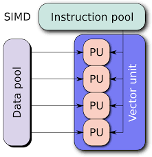
Although both multithreading and OpenMP look good and are easy to program, our optimization is not aimed at simplifying programming.
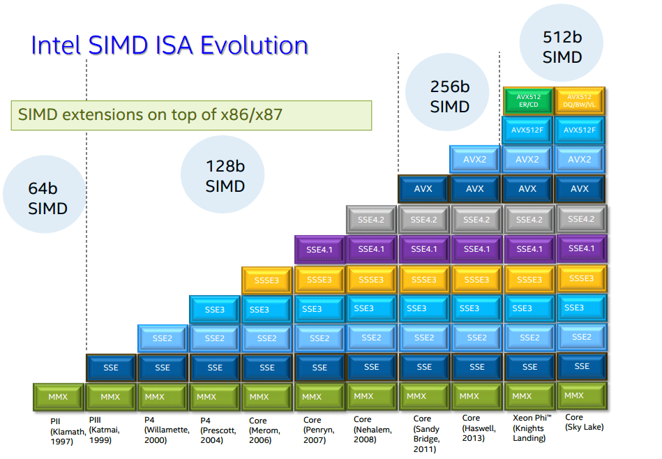
Although we complain that Intel is a toothpaste factory, the progress is getting more and more limited every year. However, new instructions are always added to new architectures. Among them are more and more powerful SIMD instructions.
SIMD is a machine instruction that can realize the operation of multiple data. On the Intel platform, the 64-bit MMX instruction set was introduced as early as 1997. In 1999, there was a 128-bit SSE instruction set. In 2011, the 256-bit AVX (Advanced Vector Extensions) instruction was introduced. Let's take a look at an example:
#include <iostream>
#include <immintrin.h> // 包含 AVX 指令集头文件

void matrix_addition_avx(float* A, float* B, float* C, int size) {


    for (int i = 0; i < size; i++) {


        for (int j = 0; j < size; j += 8) {

     // 每次处理 8 个元素(AVX 可以处理 256 位,即 8 个单精度浮点数)
            __m256 vecA = _mm256_loadu_ps(&A[i * size + j]);
            __m256 vecB = _mm256_loadu_ps(&B[i * size + j]);
            __m256 vecC = _mm256_add_ps(vecA, vecB);
            _mm256_storeu_ps(&C[i * size + j], vecC);
        }
    }
}

int main() {


    int size = 8; // 假设矩阵大小为 8x8
    float A[64] = {

     /* ... */ }; // 初始化矩阵 A
    float B[64] = {

     /* ... */ }; // 初始化矩阵 B
    float C[64] = {

     0 }; // 结果矩阵 C

    matrix_addition_avx(A, B, C, size);

    // 输出结果
    for (int i = 0; i < size; i++) {


        for (int j = 0; j < size; j++) {


            std::cout << C[i * size + j] << " ";
        }
        std::cout << std::endl;
    }

    return 0;
}
Let's explain a few statements using SIMD:
__m256 vecA = _mm256_loadu_ps(&A[i * size + j]): Load 8 floating-point numbers from matrix A (processing 256-bit data at a time), and store them in a __m256 type variable named vecA.
__m256 vecB = _mm256_loadu_ps(&B[i * size + j]): Similarly, load 8 floating-point numbers from matrix B and store them in a __m256 type variable named vecB.
__m256 vecC = _mm256_add_ps(vecA, vecB): Use the AVX instruction _mm256_add_ps to perform element-wise addition of the floating-point numbers in vecA and vecB respectively, and store the result in a variable of type __m256 named vecC.
_mm256_storeu_ps(&C[i * size + j], vecC): Store the 8 addition results in vecC back to the corresponding positions in matrix C.
This code uses the AVX instruction set to implement the addition of floating-point matrices. Note that to take full advantage of AVX's parallel processing capabilities, matrix dimensions should be multiples of 8. If the matrix size is not a multiple of 8, additional logic needs to be added to handle the remaining elements.
Later, Intel introduced the AVX2 instruction set, but there is not much optimization for our above code, and the main optimization is in integer.
The quantization and dequantization we learned in the previous section are used. This time we use the acceleration of integer calculations provided by AVX2 to achieve:
#include <iostream>
#include <immintrin.h> // 包含 AVX2 指令集头文件

void matrix_addition_avx2_int(int *A, int *B, int *C, int size) {


    for (int i = 0; i < size; i++) {


        for (int j = 0; j < size; j += 8) {

     // 每次处理 8 个元素(AVX2 可以处理 256 位,即 8 个 int32 整数)
            __m256i vecA = _mm256_loadu_si256((__m256i *)&A[i * size + j]);
            __m256i vecB = _mm256_loadu_si256((__m256i *)&B[i * size + j]);
            __m256i vecC = _mm256_add_epi32(vecA, vecB);
            _mm256_storeu_si256((__m256i *)&C[i * size + j], vecC);
        }
    }
}

int main() {


    int size = 8; // 假设矩阵大小为 8x8
    int A[64] = {

     /* ... */ }; // 初始化矩阵 A
    int B[64] = {

     /* ... */ }; // 初始化矩阵 B
    int C[64] = {

    0}; // 结果矩阵 C

    matrix_addition_avx2_int(A, B, C, size);

    // 输出结果
    for (int i = 0; i < size; i++) {


        for (int j = 0; j < size; j++) {


            std::cout << C[i * size + j] << " ";
        }
        std::cout << std::endl;
    }

    return 0;
}
The reason why we do not hesitate to quantify and convert it into an integer is that there is only _mm_add_epi32 instruction in AVX, which can only add element-wise to two 128-bit integer vectors, while _mm256_add_epi32 is 256 bits, and the amount of data is doubled.
Not just addition, AVX2 provides a series of new instructions for integer operations, such as multiplication, bit manipulation, and pack/unpack operations.
The execution throughput (throughput) of AVX2 instructions is generally 1 instruction/cycle, while AVX1 is 2 instructions/cycle. Therefore, at the same frequency, the performance of AVX2's integer addition instruction can theoretically be doubled.
At the same time, it is used in combination with other AVX2 instructions, such as _mm256_load_si256 or _mm256_store_si256, to load or store vectors from memory, which can improve the performance and bandwidth of memory access.
Later, Intel also introduced the AVX512 instruction, basically just replace 256 in AVX1 with 512:
#include <iostream>
#include <immintrin.h> // 包含 AVX-512 指令集头文件

void matrix_addition_avx512(float *A, float *B, float *C, int size) {


    for (int i = 0; i < size; i++) {


        for (int j = 0; j < size; j += 16) {

     // 每次处理 16 个元素(AVX-512 可以处理 512 位,即 16 个单精度浮点数)
            __m512 vecA = _mm512_loadu_ps(&A[i * size + j]);
            __m512 vecB = _mm512_loadu_ps(&B[i * size + j]);
            __m512 vecC = _mm512_add_ps(vecA, vecB);
            _mm512_storeu_ps(&C[i * size + j], vecC);
        }
    }
}

int main() {


    int size = 16; // 假设矩阵大小为 16x16
    float A[256] = {

     /* ... */ }; // 初始化矩阵 A
    float B[256] = {

     /* ... */ }; // 初始化矩阵 B
    float C[256] = {

    0}; // 结果矩阵 C

    matrix_addition_avx512(A, B, C, size);

    // 输出结果
    for (int i = 0; i < size; i++) {


        for (int j = 0; j < size; j++) {


            std::cout << C[i * size + j] << " ";
        }
        std::cout << std::endl;
    }

    return 0;
}
However, optimization is not always enough to pile up instructions one by one. AVX512 is a very power-hungry instruction set. At this time, we need to measure and weigh it.
For the ARM CPU used in mobile phones, NEON instructions can be used to implement SIMD functions:
#include <stdio.h>
#include <arm_neon.h>

void matrix_addition_neon(float *A, float *B, float *C, int size) {


    for (int i = 0; i < size; i++) {


        for (int j = 0; j < size; j += 4) {

     // 每次处理 4 个元素(NEON 可以处理 128 位,即 4 个单精度浮点数)
            float32x4_t vecA = vld1q_f32(&A[i * size + j]);
            float32x4_t vecB = vld1q_f32(&B[i * size + j]);
            float32x4_t vecC = vaddq_f32(vecA, vecB);
            vst1q_f32(&C[i * size + j], vecC);
        }
    }
}

int main() {


    int size = 4; // 假设矩阵大小为 4x4
    float A[16] = {

     /* ... */ }; // 初始化矩阵 A
    float B[16] = {

     /* ... */ }; // 初始化矩阵 B
    float C[16] = {

    0}; // 结果矩阵 C

    matrix_addition_neon(A, B, C, size);

    // 输出结果
    for (int i = 0; i < size; i++) {


        for (int j = 0; j < size; j++) {


            printf("%f ", C[i * size + j]);
        }
        printf("\n");
    }

    return 0;
}
For students who are new to assembly-level optimization, it may feel very fresh. However, the bigger challenge lies behind, we are going to enter the world of GPU.
GPU world
Welcome to the world of heterogeneous computing. No matter how our code was written before, it was run on the CPU.
From this moment on, no matter what technology, we are combined by two parts of code, CPU and GPU.
Let's start with CUDA, which is still the main force at present.

CUDA
CUDA 1.0 was released in 2007. The current CUDA version is 12.1.
Currently, CUDA 11.x is widely adapted, and the newer version is CUDA 11.8. Because CUDA 11.x only supports Ampere-based GPUs represented by A100. 3060, 3070, 3080, and 3090 are also Ampere-based GPUs.
The series of 2080, 2060, and 1660 are Turing architectures, corresponding to CUDA 10.x versions.
The series of 1060 and 1080 corresponds to Pascal frame, which corresponds to CUDA 8.0 version.
In CUDA, the code that runs on the GPU is called a kernel function.
Let's look at the code in its entirety first, and then explain it.
#include "cuda_runtime.h"
#include "device_launch_parameters.h"
#include <iostream>

// 矩阵加法的CUDA核函数
__global__ void matrixAdd10(int* A, int* B, int* C, int width) {


    int row = blockIdx.y * blockDim.y + threadIdx.y;
    int col = blockIdx.x * blockDim.x + threadIdx.x;
    if (row < width && col < width) {


        C[row * width + col] = A[row * width + col] + B[row * width + col];
    }
}

int main() {


    // 矩阵维度
    int width = 4;

    // 分配CPU内存
    int* A, * B, * C;
    A = (int*)malloc(width * width * sizeof(int));
    B = (int*)malloc(width * width * sizeof(int));
    C = (int*)malloc(width * width * sizeof(int));

    // 初始化A和B矩阵
    for (int i = 0; i < width; i++) {


        for (int j = 0; j < width; j++) {


            A[i * width + j] = i;
            B[i * width + j] = j;
        }
    }

    // 为GPU矩阵分配内存
    int* d_A, * d_B, * d_C;
    cudaMalloc((void**)&d_A, width * width * sizeof(int));
    cudaMalloc((void**)&d_B, width * width * sizeof(int));
    cudaMalloc((void**)&d_C, width * width * sizeof(int));

    // 将矩阵从CPU内存复制到GPU内存
    cudaMemcpy(d_A, A, width * width * sizeof(int), cudaMemcpyHostToDevice);
    cudaMemcpy(d_B, B, width * width * sizeof(int), cudaMemcpyHostToDevice);

    // 配置CUDA核函数参数
    dim3 threads(width, width);
    dim3 grid(1, 1);
    matrixAdd10 <<<grid, threads >>> (d_A, d_B, d_C, width);

    // 等待CUDA核函数执行完毕
    cudaDeviceSynchronize();

    // 将结果从GPU内存复制到CPU内存
    cudaMemcpy(C, d_C, width * width * sizeof(int), cudaMemcpyDeviceToHost);

    // 验证结果
    for (int i = 0; i < width; i++) {


        for (int j = 0; j < width; j++) {


            if (C[i * width + j] != i + j) {


                printf("错误!");
                return 0;
            }
        }
    }
    printf("矩阵加法成功!");

    // 释放CPU和GPU内存
    free(A); free(B); free(C);
    cudaFree(d_A); cudaFree(d_B); cudaFree(d_C);
}
In fact, the main function of the CPU part is relatively easy to understand. The kernel function is a bit at a loss here, such as the following two lines:
    int row = blockIdx.y * blockDim.y + threadIdx.y;
    int col = blockIdx.x * blockDim.x + threadIdx.x;
These two lines of code are used to calculate the position of the current CUDA thread in the two-dimensional matrix. In the CUDA programming model, we usually divide the problem into multiple thread blocks (block), each thread block contains multiple threads. Thread blocks and threads can be one-, two-, or three-dimensional. In this matrix addition example, we use 2D thread blocks and 2D threads.
blockIdx and blockDim represent thread block index and thread block size respectively, and they are variables of dim3 type. threadIdx represents the index of the thread and is also a variable of dim3 type. x and y denote the horizontal and vertical components of these variables, respectively.
int row = blockIdx.y * blockDim.y + threadIdx.y;
This line of code calculates the row number of the current thread in the two-dimensional matrix. blockIdx.y indicates the vertical (row direction) index of the thread block where the current thread is located, blockDim.y indicates the number of threads contained in each thread block in the vertical direction, and threadIdx.y indicates the vertical index of the current thread in the thread block . Combining these values, it is possible to calculate the current thread's row number in the entire matrix.
int col = blockIdx.x * blockDim.x + threadIdx.x;
This line of code calculates the column number of the current thread in the two-dimensional matrix. blockIdx.x indicates the horizontal (column direction) index of the thread block where the current thread is located, blockDim.x indicates the number of threads contained in each thread block in the horizontal direction, threadIdx.x indicates the horizontal index of the current thread in the thread block . Combining these values, the column number of the current thread in the entire matrix can be calculated.
With these two lines of code, we can assign each thread a specific matrix element and let it perform the corresponding addition operation. This parallel calculation method can significantly improve the calculation speed of matrix addition.
This code needs to be compiled using nvcc in the NVidia CUDA toolkit, we save it as matrix_add.cu:
nvcc -o matrix_add matrix_add.cu
./matrix_add
OpenCL
CUDA is an NVidia proprietary technology and cannot be used on other GPUs. So other manufacturers have been trying to find ways to provide similar technology. Among them, OpenCL was once the most promising. OpenCL was originally proposed by Apple and led by the Khronos Group to develop and manage the standard.
OpenCL is a framework for writing cross-platform heterogeneous computing programs. It supports writing code in C99, C++14 and C++17 languages, and can run on a variety of processors and operating systems, such as CPU, GPU , DSP, FPGA, etc.
The first version of OpenCL was released in 2008.
Let's look at an excerpt from computing matrix addition written in OpenCL.
The first is the kernel function running on the GPU, and then put it into the execution queue through enqueueNDRangeKernel.
#include <iostream>
#include <vector>
#include <CL/cl.hpp>

const char* kernelSource = R"CLC(
__kernel void matrix_add(__global const int* A, __global const int* B, __global int* C, int rows, int cols) {
    int i = get_global_id(0);
    int j = get_global_id(1);

    int index = i * cols + j;

    if (i < rows && j < cols) {
        C[index] = A[index] + B[index];
    }
}
)CLC";

int main() {


    std::vector<std::vector<int>> A = {


        {

    1, 2, 3},
        {

    4, 5, 6},
        {

    7, 8, 9}
    };

    std::vector<std::vector<int>> B = {


        {

    9, 8, 7},
        {

    6, 5, 4},
        {

    3, 2, 1}
    };

    int rows = A.size();
    int cols = A[0].size();

    std::vector<int> A_flat(rows * cols), B_flat(rows * cols), C_flat(rows * cols);
    for (int i = 0; i < rows; ++i) {


        for (int j = 0; j < cols; ++j) {


            A_flat[i * cols + j] = A[i][j];
            B_flat[i * cols + j] = B[i][j];
        }
    }

    std::vector<cl::Platform> platforms;
    cl::Platform::get(&platforms);

    cl_context_properties properties[] = {


        CL_CONTEXT_PLATFORM, (cl_context_properties)(platforms[0])(), 0
    };
    cl::Context context(CL_DEVICE_TYPE_GPU, properties);

    cl::Program program(context, kernelSource, true);

    cl::CommandQueue queue(context);

    cl::Buffer buffer_A(context, CL_MEM_READ_ONLY, sizeof(int) * rows * cols);
    cl::Buffer buffer_B(context, CL_MEM_READ_ONLY, sizeof(int) * rows * cols);
    cl::Buffer buffer_C(context, CL_MEM_WRITE_ONLY, sizeof(int) * rows * cols);

    queue.enqueueWriteBuffer(buffer_A, CL_TRUE, 0, sizeof(int) * rows * cols, A_flat.data());
    queue.enqueueWriteBuffer(buffer_B, CL_TRUE, 0, sizeof(int) * rows * cols, B_flat.data());

    cl::Kernel kernel(program, "matrix_add");
    kernel.setArg(0, buffer_A);
    kernel.setArg(1, buffer_B);
    kernel.setArg(2, buffer_C);
    kernel.setArg(3, rows);
    kernel.setArg(4, cols);

    cl::NDRange global_size(rows, cols);
    queue.enqueueNDRangeKernel(kernel, cl::NullRange, global_size);

    queue.enqueueReadBuffer(buffer_C, CL_TRUE, 0, sizeof(int) * rows * cols, C_flat.data());

    std::vector<std::vector<int>> C(rows, std::vector<int>(cols));
    for (int i = 0; i < rows; ++i) {


        for (int j = 0; j < cols; ++j) {


            C[i][j] = C_flat[i * cols + j];
        }
    }

...
Direct3D
On Windows, we all know Microsoft's DirectX, which is mainly used for game development.
As a game acceleration interface for Windows to directly access hardware, Direct X was launched as early as 1995. However, Direct X 1.0 does not support 3D, only 2D. Because the first widely used 3D accelerator card 3dfx Voodoo card was launched in 1996.
Direct3D 1.0 came out in 1996. But at this time, it is only benchmarking against the framework of OpenGL, and the relationship with GPGPU is still far away.
It was not until 2009, Direct3D 11.0 in the Windows 7 era, that it officially supported compute shaders. Direct 3D 12.0 was launched in 2015 at the same time as Windows 10.

In Direct3D 12, GPU instructions are written in the HLSL language:
// MatrixAddition.hlsl

[numthreads(16, 16, 1)]
void main(uint3 dt : SV_DispatchThreadID, uint3 gt : SV_GroupThreadID, uint3 gi : SV_GroupID) {
    // 确保我们在矩阵范围内
    if (dt.x >= 3 || dt.y >= 3) {
        return;
    }

    // 矩阵 A 和 B 的值
    float A[3][3] = {
        {1, 2, 3},
        {4, 5, 6},
        {7, 8, 9}
    };

    float B[3][3] = {
        {9, 8, 7},
        {6, 5, 4},
        {3, 2, 1}
    };

    // 计算矩阵加法
    float result = A[dt.y][dt.x] + B[dt.y][dt.x];

    // 将结果写入输出缓冲区
    RWStructuredBuffer<float> output;
    output[dt.y * 3 + dt.x] = result;
}
Then there is the operation on the CPU. To create a calculation shader, because there are many details, I will omit it and only write the main body:
#include <d3d12.h>
#include <d3dcompiler.h>
#include <iostream>

// 创建一个简单的计算着色器的 PSO
ID3D12PipelineState* CreateMatrixAdditionPSO(ID3D12Device* device) {


    ID3DBlob* csBlob = nullptr;
    D3DCompileFromFile(L"MatrixAddition.hlsl", nullptr, nullptr, "main", "cs_5_0", 0, 0, &csBlob, nullptr);

    D3D12_COMPUTE_PIPELINE_STATE_DESC psoDesc = {

    };
    psoDesc.pRootSignature = rootSignature; // 假设已创建好根签名
    psoDesc.CS = CD3DX12_SHADER_BYTECODE(csBlob);

    ID3D12PipelineState* pso = nullptr;
    device->CreateComputePipelineState(&psoDesc, IID_PPV_ARGS(&pso));

    csBlob->Release();
    return pso;
}

// 执行矩阵加法计算
void RunMatrixAddition(ID3D12GraphicsCommandList* commandList, ID3D12Resource* outputBuffer) {


    commandList->SetPipelineState(matrixAdditionPSO);
    commandList->SetComputeRootSignature(rootSignature);
    commandList->SetComputeRootUnorderedAccessView(0, outputBuffer->GetGPUVirtualAddress());
    // 分发计算着色器,设置线程组的数量
    commandList->Dispatch(1, 1, 1);

    // 确保在继续之前完成计算操作
    commandList->ResourceBarrier(1, &CD3DX12_RESOURCE_BARRIER::UAV(outputBuffer));
}

int main() {


    // 初始化 DirectX 12 设备、命令队列、命令分配器等...
    // ...

    // 创建根签名、PSO 和计算着色器相关资源
    // ...

    // 创建输出缓冲区
    ID3D12Resource* outputBuffer = nullptr;
    device->CreateCommittedResource(
        &CD3DX12_HEAP_PROPERTIES(D3D12_HEAP_TYPE_DEFAULT),
        D3D12_HEAP_FLAG_NONE,
        &CD3DX12_RESOURCE_DESC::Buffer(3 * 3 * sizeof(float)),
        D3D12_RESOURCE_STATE_UNORDERED_ACCESS,
        nullptr,
        IID_PPV_ARGS(&outputBuffer)
    );

    // 创建并执行命令列表
    ID3D12GraphicsCommandList* commandList = nullptr;
    device->CreateCommandList(0, D3D12_COMMAND_LIST_TYPE_DIRECT, commandAllocator, nullptr, IID_PPV_ARGS(&commandList));

    RunMatrixAddition(commandList, outputBuffer);

    // 关闭命令列表并执行
    commandList->Close();
    ID3D12CommandList* commandLists[] = {

    commandList};
    commandQueue->ExecuteCommandLists(_countof(commandLists), commandLists);

    // 同步 GPU 和 CPU
    // ...

    // 从输出缓冲区中读取结果
    float result[3][3] = {

    };
    void* mappedData = nullptr;
    outputBuffer->Map(0, nullptr, &mappedData);
    memcpy(result, mappedData, sizeof(result));
    outputBuffer->Unmap(0, nullptr);

    // 输出结果
    for (int i = 0; i < 3; ++i) {


        for (int j = 0; j < 3; ++j) {


            std::cout << result[i][j] << " ";
        }
        std::cout << std::endl;
    }

    // 清理资源
    // ...
}
Vulkan

Vulkan is led by the Khronos Group to develop and manage standards and is the successor to OpenGL. Its earliest technology came from AMD.
Vulkan is a framework for writing cross-platform graphics and computing programs. It supports writing code in C and C++ languages and can run on a variety of processors and operating systems, such as CPU, GPU, DSP, FPGA, etc.
Version 1.0 of Vulkan was released in 2016.
By default, Vulkan uses glsl with compute pipeline:
#version 450
#extension GL_ARB_separate_shader_objects : enable

layout (local_size_x = 16, local_size_y = 16, local_size_z = 1) in;

layout (binding = 0) readonly buffer InputA {
    float dataA[];
};

layout (binding = 1) readonly buffer InputB {
    float dataB[];
};

layout (binding = 2) writeonly buffer Output {
    float dataC[];
};

void main() {
    uint index = gl_GlobalInvocationID.x + gl_GlobalInvocationID.y * gl_NumWorkGroups.x * gl_WorkGroupSize.x;
    dataC[index] = dataA[index] + dataB[index];
}
Then, in the host program, complete the following steps:
- Initialize Vulkan instance and physical/logical devices.
- Create a Vulkan compute pipeline, load and compile compute shaders.
- Create Vulkan buffers for input matrices A and B and output matrix C.
- Copy the input matrix data to the input buffer.
- Create descriptor set layouts and descriptor pools to describe resource bindings in shaders.
- Create a descriptor set and bind input/output buffers to the descriptor set.
- Creates a Vulkan command buffer to record commands for compute shader scheduling.
- Start recording the command buffer, and call vkCmdBindPipeline and vkCmdBindDescriptorSets to bind the computation pipeline and descriptor sets to the command buffer.
- Use vkCmdDispatch to schedule a compute shader to perform matrix addition.
- End the command buffer recording and submit the command buffer to the Vulkan queue.
- Wait for the queue execution to complete and copy the output buffer's data back to host memory.
- Clean up Vulkan resources.
The specific code is not listed in detail.
The approximate code structure is:
// Vulkan实例、设备、命令池、队列
VkInstance instance;
VkDevice device;
VkCommandPool commandPool;
VkQueue queue;

// 矩阵维度
const int width = 4;

// 顶点缓冲区对象
VkBuffer vertexBuffer;
VkDeviceMemory vertexBufferMemory;

// 结果缓冲区对象
VkBuffer resultBuffer;
VkDeviceMemory resultBufferMemory;

// 着色器模块和管线
VkShaderModule shaderModule;
VkPipeline pipeline;

// 创建顶点缓冲区
// 向缓冲区填充矩阵A和B
// ...

// 创建结果缓冲区
// 向缓冲区映射内存
void* resultData;
vkMapMemory(device, resultBufferMemory, 0, sizeof(int) * 4 * 4, 0, &resultData);

// 创建着色器模块(矩阵加法着色器)
const char* shaderCode = "上面的glsl";
shaderModule = createShaderModule(shaderCode);

// 创建图形管线
// ...

// 记录命令
VkCommandBuffer commandBuffer;
VkCommandBufferAllocateInfo commandBufferAllocateInfo = ...;
vkAllocateCommandBuffers(commandPool, &commandBufferAllocateInfo, &commandBuffer);

// 开始记录命令
vkBeginCommandBuffer(commandBuffer, &beginInfo);

// 绑定顶点缓冲区和结果缓冲区
vkCmdBindVertexBuffers(commandBuffer, 0, 1, &vertexBuffer, &offset);
vkCmdBindBuffer(commandBuffer, 1, 0, resultBuffer, &offset);

// 绘制
vkCmdDraw(commandBuffer, 4, 1, 0, 0);

// 结束记录命令
vkEndCommandBuffer(commandBuffer);

// 提交命令并执行
VkSubmitInfo submitInfo = ...;
vkQueueSubmit(queue, 1, &submitInfo, VK_NULL_HANDLE);
vkQueueWaitIdle(queue);

// 读取结果矩阵
for (int i = 0; i < width; i++) {


    for (int j = 0; j < width; j++) {


        int result = ((int*)resultData)[i * width + j];
        printf("%d ", result);
    }
    printf("\n");
}

// 释放Vulkan资源
...
WebGPU
WebGPU is a front-end GPU technology that has just been supported by the Chrome browser.
WebGPU is a framework for writing cross-platform graphics and computing programs. It supports writing code in JavaScript and WebAssembly, and can run on multiple browsers and operating systems, such as Chrome, Firefox, Safari, etc. WebGPU is a standard developed and managed by W3C's GPU for the Web working group and is the successor of WebGL.
As we saw earlier, CUDA derived from NVidia technology, OpenCL derived from Apple technology, DirectX derived from Microsoft technology, and Vulkan derived from AMD technology are flourishing on the desktop and server side. On the mobile side, it is natural that fighting between dragons and tigers is indispensable.
Apple was the first to propose the idea of WebGPU. In February 2016, Apple put forward a proposal called Web Metal, which aimed to port the concept of Metal API to the Web platform.
In February 2017, Microsoft Corporation put forward a proposal called Web D3D, which aims to port the concept of Direct3D 12 API to the Web platform.
In August 2017, the Mozilla Corporation put forward a proposal called Obsidian, which aims to create an abstraction layer based on the Vulkan API.
After several disputes, Google put forward a proposal called NXT, which aims to create an abstraction layer based on Vulkan, Metal and Direct3D 12 API.
In April 2018, the W3C working group decided to use NXT as the starting point for the draft specification and renamed it WebGPU.
Since it is an abstraction layer, the shader language is not suitable whether it uses SPIR-V, Vulkan's GLSL, DirectX's HLSL or Apple's Metal Shading Language.
So in 2019, the WebGPU community group proposed a new shader language proposal called WebGPU Shading Language (WGSL), which aims to create a text format based on SPIR-V to provide a safe, portable, easy-to-use and an easy-to-implement shader language.
The following code shows the process, and the browser officially supports it at this moment. After the bullets fly for a while and the browser is officially launched, we will talk about it later.
Look at the picture below: the specification of WebGPU has not been released yet. The specification of WGSL also has no final release.

js
// 获取WebGPU adapter和设备
const adapter = await navigator.gpu.requestAdapter();
const device = await adapter.requestDevice();

// 矩阵维度
const width = 4;

// 创建缓冲区 - 用作顶点缓冲区和结果缓冲区
const vertexBuffer = device.createBuffer({


  size: width * width * 4 * Int32Array.BYTES_PER_ELEMENT,
  usage: GPUBufferUsage.VERTEX | GPUBufferUsage.STORAGE
});

// 获得缓冲区映射 - 填充矩阵A和B
const vertexBufferMapping = await vertexBuffer.map();
new Int32Array(vertexBufferMapping).fill(/* A和B矩阵 */);
vertexBuffer.unmap();

// 着色器代码
const shaderCode = `
  kernel void addMatrices(device int* a [[buffer(0)]],
                          device int* b [[buffer(1)]],
                          device int* c [[buffer(2)]]) {
    const int width = 4;
    int tid = threadIdx.x * 4 + threadIdx.y;
    if (tid < width * width) {
      c[tid] = a[tid] + b[tid];
    }
  }
`;

// 创建着色器模块
const shaderModule = device.createShaderModule({


  code: shaderCode
});

// 运行着色器 - 执行矩阵加法
const pipeline = device.createComputePipeline({


  compute: {


    module: shaderModule,
    entryPoint: "addMatrices"
  }
});
const passEncoder = device.createCommandEncoder();
const computePass = passEncoder.beginComputePass();
computePass.setPipeline(pipeline);
computePass.setBuffer(0, vertexBuffer);
computePass.setBuffer(1, vertexBuffer);
computePass.setBuffer(2, vertexBuffer);
computePass.dispatch(1);
computePass.endPass();
device.queue.submit([passEncoder.finish()]);

// 读取结果
const result = new Int32Array(
  await vertexBuffer.mapRead()
);
// 打印结果矩阵
...

// 释放资源
summary
Although the details have not been covered yet, this article opened the door for us to SIMD and GPU programming.