Introductory Guide to Deep Learning in 2023 (17) - Hardware Acceleration Technology for Deep Learning

With the previous knowledge, everyone must have a deeper understanding of computing power requirements.

In addition to using general-purpose devices such as CPUs and GPUs, using dedicated hardware for acceleration is a choice that everyone can think of.

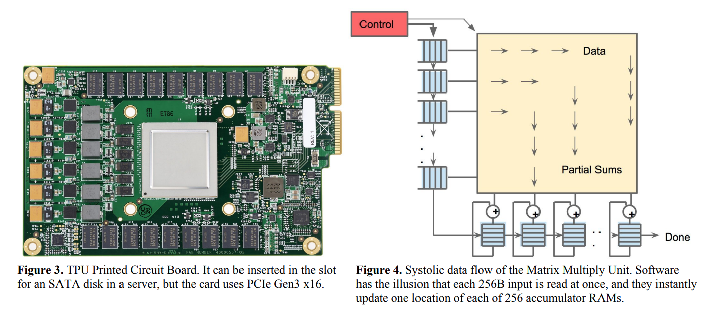
The representative device is the TPU we just used in the previous section. The following figure is what the TPU looks like and its structure:

So, why is the TPU designed to take matrix multiplication as the core? Let's start with the principles of deep learning.

Computational Methods for Neural Networks and Attention

The basic computational unit of an artificial neural network is a neuron. The structure of each neuron is shown in the figure below:

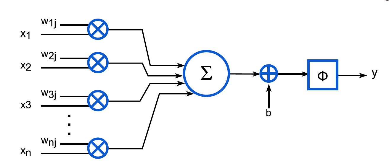
Expressed by the formula is:

$y_j=\Phi\left(\sum_{k=0}^{n-1} x_k w_{k j}+b\right)$

Among them, $x_k$ is the input, $w_{kj}$ is the weight, $b$ is the bias, $\Phi$ is the activation function, $y_j$ is the output.
We can see that the calculation of each neuron is a matrix multiplication plus a bias, and then an activation function.

Let's review the structure diagram of the multi-head self-attention model before:

We can see that the main calculations are still matrix multiplication and addition.

$Query: Q_i = X * W_i^{Q}$

$Key: K_i = X * W_i^{K}$

$Value: V_i = X * W_i^{V}$

$Attention weight: A_i = softmax(Q_i * K_i^T / sqrt(d_k))$

$Export: O_i = A_i * V_i$

With the above foundation, let's take a look at the structure diagram of TPU:

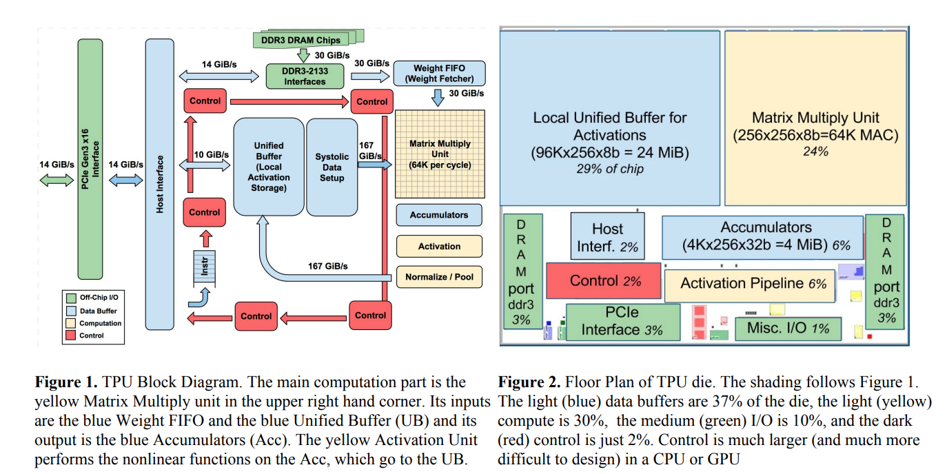
It can be seen that the matrix multiplication unit in the upper right corner occupies a quarter of the space, and the local cache in the upper left part constitutes the most important part of the TPU.

The MAC in the above figure is the abbreviation of Multiply-and-accumulate, which means multiplication plus accumulation operation. That is to say, on the original TPU, 64K multiplication and addition operations can be performed per instruction cycle.

hardware approximation method

Matrix multiplication is a very time-consuming operation, and in deep learning, we don't need very accurate results. Therefore, we can use some approximate methods to speed up the operation of matrix multiplication.

Similar to the quantization and pruning methods we learned before, we can also use quantization and computational simplification methods on the hardware method. In addition, in hardware design, we can also use approximate computing units instead of precise computing devices.

There are three main ways to approximate the calculation unit, the first is to use an approximate addition multiplier, the second is to convert multiplication into addition by using logarithms, and the last is to simply remove the multiplier.

We have already introduced quantization in detail before, so I won't repeat it here. We mainly introduce the latter two methods, that is, computational simplification and approximate computational unit.

Computational simplification - skip

The first way to calculate simplification is to skip counting.

In the large model, due to the large amount of data, there are actually many data that are 0, or very close to 0. These data have very little influence on the final result, so we can skip the calculation of these data directly.

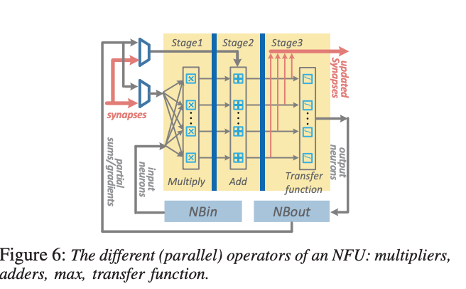
We can design a calculation unit that skips data close to 0 as follows:

Computational Simplification - Memory

The second method of calculation simplification is memory, which means that we can save the previous calculation results and use them directly next time. Isn't this the idea of dynamic programming? The efficiency of this approach depends on the similarity of the inputs (i.e. how often substitutions occur) and the complexity of the computations being eliminated.

The higher the similarity of the inputs, the higher the computational complexity that is eliminated, the more efficient this approach is.

For example, the paper "(Pen-) Ultimate DNN Pruning" proposes a two-step pruning method, which first removes redundant nodes by performing PCA analysis on the output of each layer, and then removes redundant nodes by considering its relative The contributions of other connections are used to remove the remaining unimportant connections.

Approximate Computing Unit - Approximate Multiply Adder

In the realization of approximate circuits, a more effective method is the Cartesian Genetic Programming (GCP) method. The most basic implementation looks like this:

Cartesian Genetic Programming (CGP) is a form of genetic programming that uses graphical notation to encode computer programs. It originated from a method of evolving digital circuits developed by Julian F. Miller and Peter Thomson in 1997. It is called "Cartesian" because it uses the nodes of a two-dimensional grid to represent a program

Genetic programming is a heuristic search technique used to optimize or discover computer programs that can perform user-defined tasks. Basic genetic programming systems use a genetic algorithm, a search algorithm that operates on the principles of biological evolution, including heredity, variation, natural selection, and recombination.

In Cartesian genetic programming, a program is represented by a graph consisting of nodes, each node representing a function or operation. These nodes are arranged in a two-dimensional grid to form a computational flow, which is the path through which computation flows from input nodes to output nodes. In this way, CGP is able to evolve complex programs capable of accomplishing specific tasks.

Cartesian genetic programming generates multipliers that satisfy the given worst-case error constraints and ensure that multiplications of 0 are always correct. It employs an iterative optimization process to determine the error constraints generated by the approximate multiplier in the CGP optimization to meet a threshold for inference accuracy loss. And, in an iterative process, after replacing the exact multipliers with approximate multipliers, the network is retrained to obtain the best quality results.

Starting with the basic paper "Design of power-efficient approximate multipliers for approximate artificial neural networks." using GCP, there are a series of improvements later, such as using weighted mean error distance (WMED) for error measurement. When computing WMED, the importance of each error is determined by the probability mass function of the network weight distribution.

The paper "Neural Networks with Few Multiplications" proposes a two-step approach: first, the authors convert the multiplication operations required to compute the hidden state into sign changes by stochastically binarizing weights. Second, in the process of backpropagating error derivatives, in addition to binarizing weights, the authors also quantize the representation of each layer, converting the remaining multiplication operations into binary displacements.
In addition, after using Ternary Connect, Quantized Backprop and Batch Normalization, the error rate can be reduced to 1.15%, which is 1.33% higher than the error rate of full-precision training. to be low. This shows that even with most of the multiplications removed, the performance of this method is still comparable to full-precision training, or even improved slightly. The performance improvement may be due to the regularization effect brought about by random sampling.

The method proposed in the paper "ALWANN: Automatic layer-wise approximation of deep neural network accelerators without retraining" consists of two parts: the first part is to convert a fully trained DNN to use 8-bit weights and 8-bit multiplication in the convolutional layer operation of multipliers; the second part is to select a suitable approximate multiplier for each computational unit from a library of approximate multipliers, so that (i) one approximate multiplier can serve multiple layers, (ii) the overall classification Errors and energy consumption are minimized.

The figure below is the architecture diagram of the Cambrian DaDianNao chip computing approximate multiplication.

The paper "Design automation of approximate circuits with runtime reconfigurable accuracy" proposes an automatic design framework that can generate approximate circuits with runtime reconfigurable accuracy. The method of the paper consists of two parts: the first part is to use the genetic algorithm to approximate the given circuit at the gate level, so as to reduce the overhead of the circuit without affecting the correctness of the function; the second part is to add a programmable Reconfiguring the unit allows the circuit to switch between different precision levels at runtime according to application requirements and environmental conditions.

Approximate Computing Unit - Multiplier-less Design

Having seen the dedicated hardware TPU, DaDianNao, let's look at a new device FPGA.

The paper "AddNet: Deep Neural Networks Using FPGA-Optimized Multipliers"
proposes a method of using FPGA-optimized multipliers to implement deep neural networks, called AddNet. The approach utilizes reconfigurable constant coefficient multipliers (RCCMs), which can implement multiplication with adders, subtractors, shifts, and multiplexers (MUX), to be highly optimized on FPGAs. The authors designed a series of RCCMs suitable for FPGA logic elements to ensure their efficient utilization. To reduce the information loss caused by quantization, the authors also develop a novel training technique that maps possible coefficient representations of RCCM onto neural network weight parameter distributions. This makes it possible to maintain high accuracy when using RCCM on hardware.

Similarly, the main point of the paper "Energyefficient neural computing with approximate multipliers" is to propose a method for energy-efficient neural computing using approximate multipliers. The approach takes advantage of the error resilience of neural network applications, using the concept of computation sharing to enable low-precision multiplication operations that save silicon area or increase throughput. The authors design an approximate multiplier that uses adders, subtractors, shifts, and multiplexers (MUXs) to implement multiplication operations that are highly optimized on FPGAs. Use multiplier-less neurons by replacing multipliers with simplified shift and add operations, controlled by a single unit. So-called alphabet set multipliers (ASMs) consist of banks of precalculators based on some small sequence of bits called alphabets ({1, 2, 3, 5, . . . }), an adder, and one or more select, shift, and control logic to compute low-order multiples of the input. The size of the alphabet defines the accuracy and energy gain of the ASM. Finally, effective retraining is performed to adjust the weights and mitigate the accuracy drop due to ASMs.

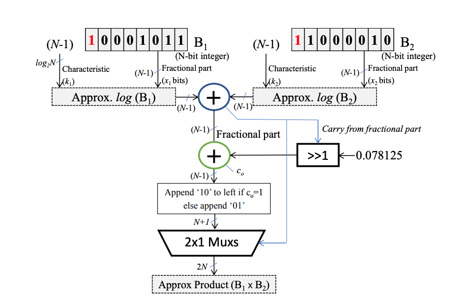
Approximate Computing Unit - Approximate Logarithmic Multiplier

The research on turning multiplication into addition by using logarithms and exponents has a long history. John N. Mitchell proposed a computer multiplication and division using binary logarithms in his 1962 paper "Computer multiplication and division using binary logarithms". Methods of multiplication and division. This method allows approximately determining the logarithm of a binary number itself, by simple shifting and counting. Multiplication or division can be done with a simple addition or subtraction and shift operation.

The following is a schematic diagram of an improved algorithm. There are many formulas involved, so I won’t go into details:

summary

This section just wants to popularize it for everyone, because the tolerance of the neural network has brought a lot of space for various hardware optimizations. Although the current training of large models can basically only use NVidia GPUs, there must still be a lot of room for optimization in future training and inference.

Please pay attention to the development of hardware at any time. If you find that hardware that can be used in your own business scenarios can save costs or improve performance, you must keep an open mind and try it.