LSTM---long short-term memory recurrent neural network is a very commonly used neural network. Its characteristic is that the network introduces the concept of long-term memory and short-term memory, so it is suitable for some regression and classification with context, such as temperature prediction or semantic understanding. From the perspective of using pytorch to construct a model, the model will have some differences compared with the general model, especially in the setting of parameters. This article tries to explain some of my understanding in a relatively popular way.
This article mainly refers to: comprehensive understanding of LSTM network and input, output, hidden_size and other parameters
LSTM and general recurrent neural network
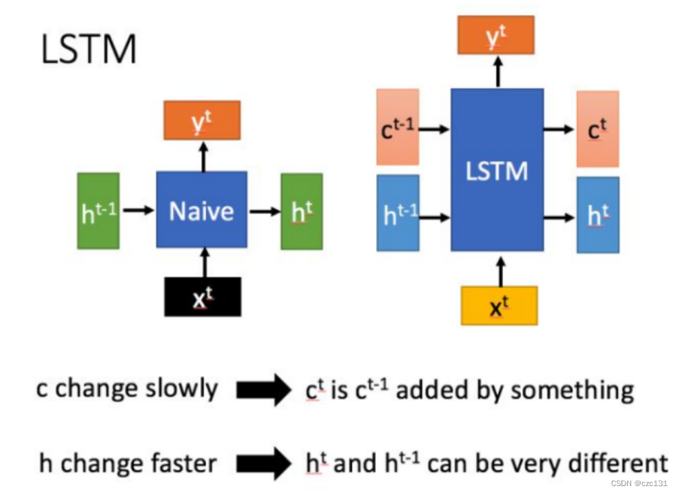
As shown in the figure below, h[t] is understood as the state passed to time t, which is short-term and changes quickly. c[t] is unique to LSTM and is understood as long-term memory. In contrast, the general network is to pass this state to the next state, that is, from h[t-1] to h[t] --- short-term memory transfer, and LSTM except h[t-1] There is also a relatively slow-changing c[t] transfer to h[t], and this node is mainly used to store information, so the general network can only see the information of the previous few close points at the current point. And LSTM can see the memory of a long period of time before, which is context understanding.
How to implement delivery
Then how to realize long-term and short-term memory, LSTM introduces the concept of gate, the general network input x, after some changes, the output result is over, but LSTM needs to perform various processing on x.
As shown in the figure below, there are two horizontal lines running through the time series. The upper one is the long-term memory c, and the lower one is the short-term memory h, which represents the gate control status ![]() value, which is a ratio. Forgetting is required, and σ represents the sigmoid activation function. After this, a number ∈ [0,1] can be obtained, which is the forgetting ratio. The input x comes in and is first mixed with the short-term memory of the previous moment , and then goes through three gating operations. First look at the first one on the upper left, the long-term memory c has passed, so the part of the long-term memory is forgotten; then look at the middle one, it shows the part that is to be forgotten in the short-term memory, and then go up and sum with the long-term memory to form a new long-term memory Time memory; the last is the bottom right corner, this is the current long-term memory and short-term memory for tanh activation operation, so that we can get the current new short-term memory, and then the long-term memory and short-term memory continue to affect the following , forming a recurrent network.
value, which is a ratio. Forgetting is required, and σ represents the sigmoid activation function. After this, a number ∈ [0,1] can be obtained, which is the forgetting ratio. The input x comes in and is first mixed with the short-term memory of the previous moment , and then goes through three gating operations. First look at the first one on the upper left, the long-term memory c has passed, so the part of the long-term memory is forgotten; then look at the middle one, it shows the part that is to be forgotten in the short-term memory, and then go up and sum with the long-term memory to form a new long-term memory Time memory; the last is the bottom right corner, this is the current long-term memory and short-term memory for tanh activation operation, so that we can get the current new short-term memory, and then the long-term memory and short-term memory continue to affect the following , forming a recurrent network.
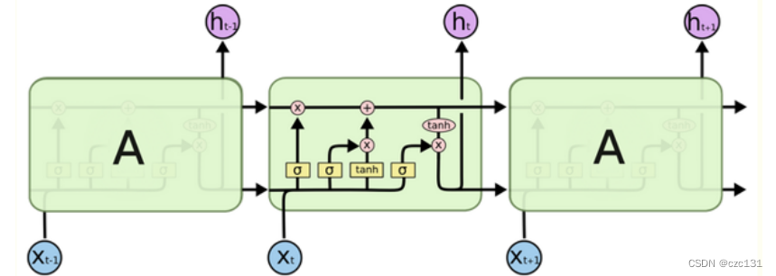
This process is actually very vivid. From the perspective of reading a book, a piece of text we see is actually input x at the current time. Long-term memory includes the content read earlier, while short-term memory is the content just read. When we read a piece of content, we will first combine the content we just read, which is the mixture of x and the short-term memory of the previous moment . The gate on the upper left indicates long-term memory forgetting , which is the forgetting of our memory; the tanh operation in the middle is the current Of course, it is impossible to remember all of them, so I enter the long-term memory through the gated forgetting part in the middle ; then I need to combine the long-term memory and the current content context to understand the current reading content, and generate New understanding, then it is tanh activation ; the last forgotten part becomes the "just read" in the next moment. From a macro point of view, the longer you read the content, the more you forget it. This is also in line with the fact that the farther away the memory is, the less affected it is during the transfer process.
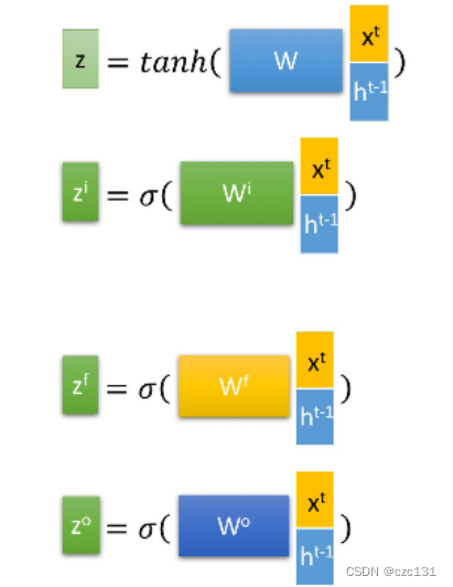
When it comes to implementation, it is the following operations, which will not be expanded.
The figure below shows the structure of an overall LSTM network, that is, the changes experienced by a sequence input and output, which is very helpful for understanding the parameters behind. The overall input is one of the time series of all data, a sequence contains several units, and the horizontal distribution is similar to a sentence selected from an article, which contains several words; the vertical distribution is the continuous deepening of the network layer, that is, the general Multilayer Neural Architecture of Networks. Each blue box is a neuron. Observe that one of the neurons receives the long-term and short-term influence of the same layer of the previous sequence, and at the same time receives the short-term influence of the previous layer of this sequence, and continues to influence the next layer. One layer and the sequence below (directly affects the next one, indirectly affects everything after the next one). The final output contains the output features of each sequence, which is essentially recording the short-term memory of each sequence and finally splicing them together. And hn and cn record the short-term memory and long-term memory of the nth sequence.

LSTM network parameter understanding
Now comes the time to use pytorch to construct the LSTM network. The code is not difficult to find, but it is often difficult to understand the meaning of the parameters inside. I have not found a very satisfying analysis myself. Let me analyze some incomprehensible ones in detail from my perspective. parameters.
   def __init__(self, input_size, hidden_size, num_layers, output_size, batch_size, seq_length) -> None:
        super(Net, self).__init__()
        self.input_size = input_size
        self.hidden_size = hidden_size
        self.num_layers = num_layers
        self.output_size = output_size
        self.batch_size = batch_size
        self.seq_length = seq_length
        self.num_directions = 1  # 单向LSTM

        self.lstm = nn.LSTM(input_size=input_size, hidden_size=hidden_size, num_layers=num_layers,
                            batch_first=True)  # LSTM层
Assuming that a simple LSTM model is constructed above, the explanation of all parameters is given below.
seq_length = 3 # Time step, you can set it yourself
input_size = 3 # Input dimension size
num_layers = 6 # Network layer number
hidden_size = 12 # Hidden layer size
batch_size = 64 # Batch number
output_size = 1 # Output dimensionnum_directions=1 # means one-way LSTM, equal to 2 is two-way LSTM
input_size and output_size are well understood, that is, the number of dimensions of x and y, I don’t need to explain much, num_directions means the number of directions of LSTM, I haven’t studied this, maybe both directions are positive and negative?
seq_length is how many units each time series contains, or how many pieces of data it contains. If it is 3, then pack the data of 3 moments into one piece each time, and put a corresponding y label as a piece of data, that is, a sequence seq.
num_layers is the number of layers of the network, and the depth of the overall structure above is the number of layers here.
The batch-size indicates how many batches of data are sent in at a time for training. I personally like to understand it as the number of superimposed layers . In general networks, such as image recognition, it is to train multiple pictures at a time, which is equivalent to batch-size The pictures are superimposed together, and then the parameters are optimized, which is similar in LSTM, which is to send multiple batches of time series at a time for training .
Finally, hidden-size , hidden-size is beginning to bother me, this is the size of the hidden layer hn, which is the size of the short-term memory (number of columns). Here it needs to be understood in combination with the previous figure. Every time x data comes in, it does not directly enter the network, but is mixed with the hidden layer, that is, x[n] and h[n] are superimposed, and the column The numbers are added together, and then sent to the model training, so the number of columns of the weight parameters of the real network model must be hidden_size+input_size, after passing through the network and forming a new short-term memory h[n+1], the number of columns at this time is It is hidden_size, and finally mixed with x[n+1] to form a new short-term memory and propagate downward .
The following two parameter matrix sizes are combined with the overall diagram for understanding:
(h[n], c[n])
h[n] shape:(num_layers * num_directions, batch_size, hidden_size)
c[n] shape:(num_layers * num_directions, batch_size, hidden_size)
As above, this is the specific size of the entire hidden layer state, which are long-term memory and short-term memory, which are roughly the same. Take h[n], which is the overall short-term memory of the nth layer, as an example. The overall memory is actually the collection of short-term memory in each layer at all moments of this time series . Combined with the graph, one column has num_layers layers, and each layer There is an output with a size of hidden_size, then the superposition becomes num_layers hidden_size lengths, and each hidden_size has a superposition of a batch_size layer, and the bidirectional LSTM needs to be *2.
output
output.shape: (seq_length, batch_size, hidden_size * num_directions)
Looking at the output again, combined with the diagram, we can see that output is the output set of the short-term memory of each node in the last layer in a time series, which can be understood as the set of short-term memory of each node, and the length is the time in the sequence The number seq_length, each moment is the superposition of hidden_size, batch_size layers. Pay attention to the distinction, this is only the output of one of the sequences during the training process, which is equivalent to the x output in a set of xy relationships, not the final output, and the final output needs to be feature mapped .
On the whole, output is the final collection of short-term memory at each moment, reflecting the overall characteristics of this period of time sequence, and the hidden layers h[n] and c[n] are the long and short time Memories, which reflect the characteristics of this moment, are often used as predictions or classifications.