Table of contents
In recent years, with the development of models based on the Self-Attention structure, especially the Transformer model, the development of natural language processing models has been greatly promoted. Due to the computational efficiency and scalability of Transformers, it has been able to train models of unprecedented scale with over 100B parameters.
ViT is the fusion of natural language processing and computer vision. It can still achieve good results on image classification tasks without relying on convolution operations.
Model structure
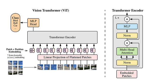
The main structure of the ViT model is based on the Encoder part of the Transformer model (the order of some structures has been adjusted, such as: the position of Normalization is different from the standard Transformer), and its structure diagram [1] is as follows: Model characteristics The ViT model is mainly used in the field of
image
classification . Therefore, compared with the traditional Transformer, its model structure has the following characteristics:
After the original image of the data set is divided into multiple patches, the two-dimensional patch (regardless of the channel) is converted into a one-dimensional vector, plus the category vector with the position vector as model input.
The Block structure of the main body of the model is based on the Transformer's Encoder structure, but the position of Normalization has been adjusted. Among them, the most important structure is still the Multi-head Attention structure.
The model is connected to the fully connected layer after Blocks stacking, accepting the output of the category vector as input and used for classification. Usually, we call the last fully connected layer Head, and the Transformer Encoder part is backbone.
The following will explain in detail the implementation of the ImageNet classification task based on ViT through code examples.
If you are interested in MindSpore, you can follow the Shengsi MindSpore community


1. Environmental preparation
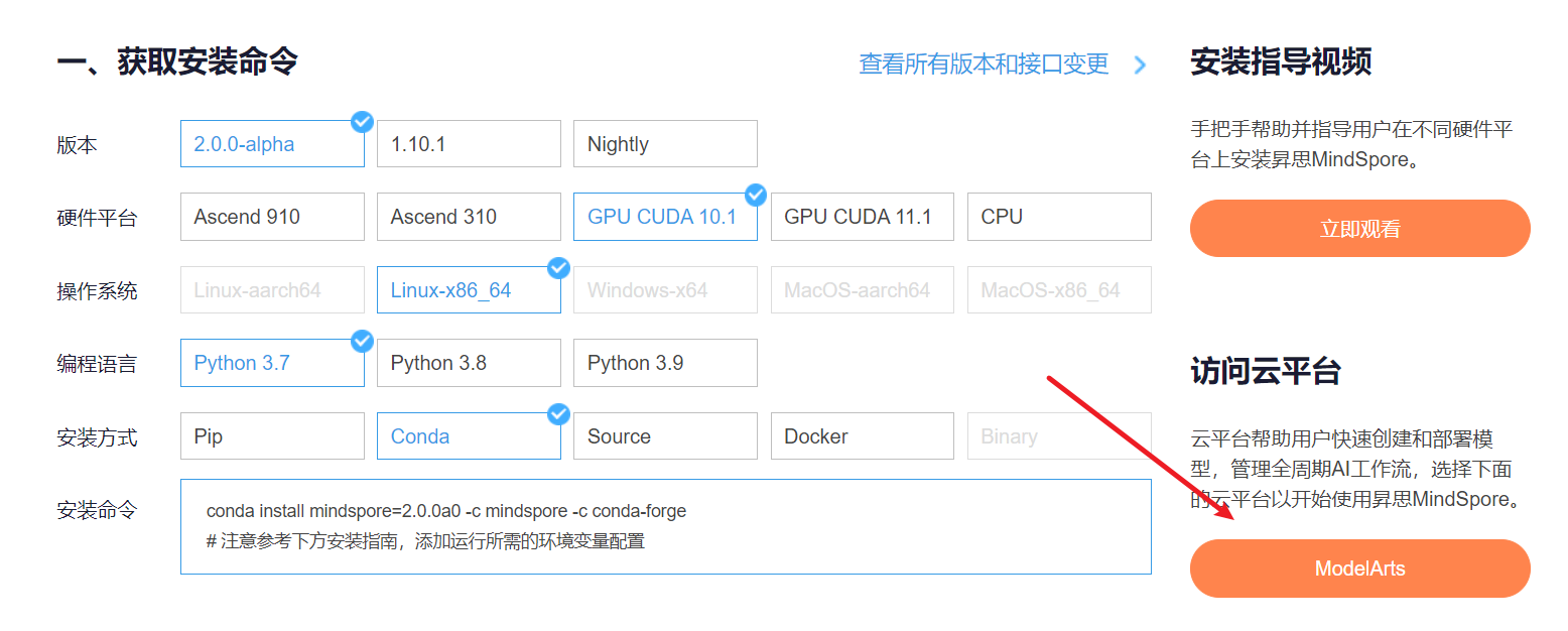
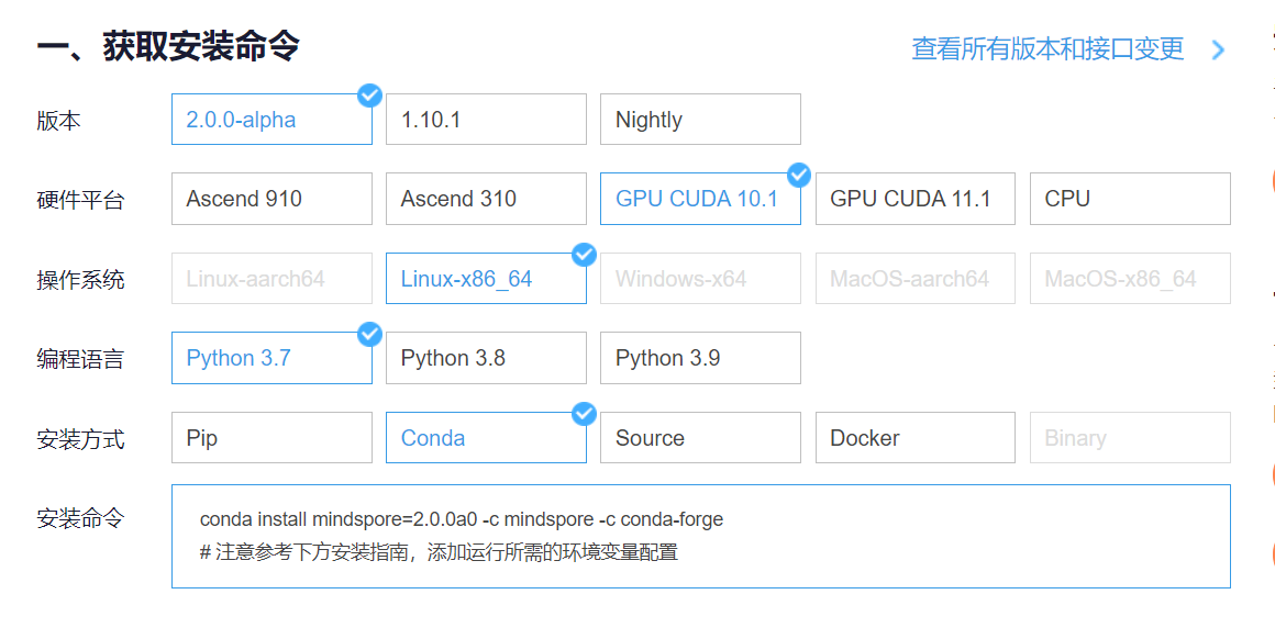
1. Enter ModelArts official website
The cloud platform helps users quickly create and deploy models, and manage full-cycle AI workflows. Select the following cloud platform to start using Shengsi MindSpore, get the installation command , install MindSpore2.0.0-alpha version, and enter the ModelArts official website in the Shengsi tutorial
Choose CodeLab below to experience it immediately

Wait for the environment to be built

2. Use CodeLab to experience Notebook instances
Download NoteBook sample code , Vision Transformer image classification , .ipynbas sample code

Select ModelArts Upload Files to upload .ipynbfiles


Select the Kernel environment

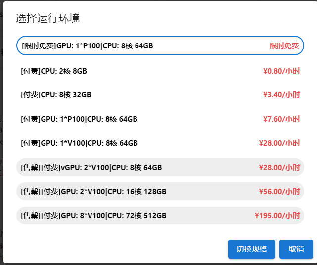
Switch to the GPU environment, switch to the first time-limited free
Enter Shengsi MindSpore official website , click on the installation above

get install command
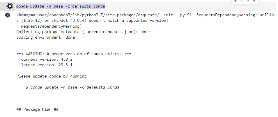
Back in the Notebook, add the command before the first block of code

conda update -n base -c defaults conda
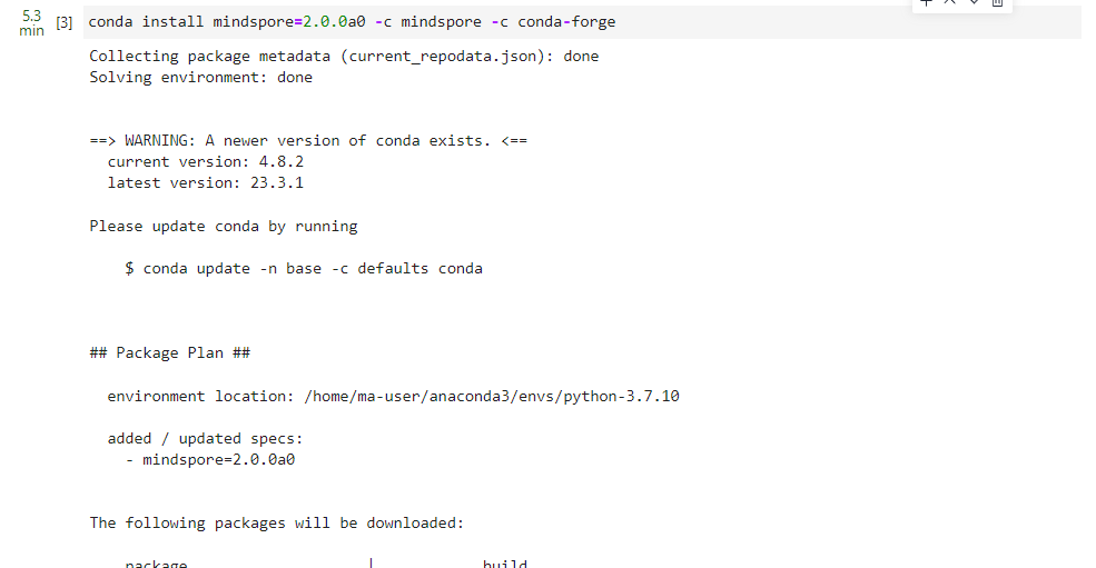
Install MindSpore 2.0 GPU version
conda install mindspore=2.0.0a0 -c mindspore -c conda-forge
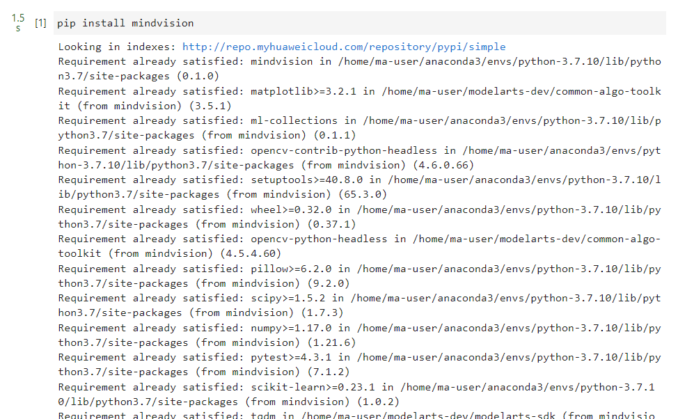
install mindvision
pip install mindvision
installdownloaddownload
pip install download
2. Environment preparation and data reading
Before starting the experiment, please ensure that the Python environment and MindSpore have been installed locally.
First of all, we need to download the data set of this case. You can download the complete ImageNet data set through http://image-net.org. The data set used in this case is a subset selected from ImageNet.
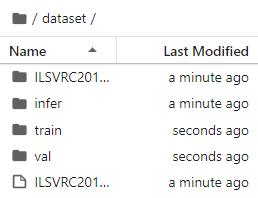
When you run the first piece of code, it will be downloaded and decompressed automatically. Please make sure that your dataset path has the following structure.
.dataset/
    ├── ILSVRC2012_devkit_t12.tar.gz
    ├── train/
    ├── infer/
    └── val/
from download import download

dataset_url = "https://mindspore-website.obs.cn-north-4.myhuaweicloud.com/notebook/datasets/vit_imagenet_dataset.zip"
path = "./"

path = download(dataset_url, path, kind="zip", replace=True)

import os

import mindspore as ms
from mindspore.dataset import ImageFolderDataset
import mindspore.dataset.vision as transforms


data_path = './dataset/'
mean = [0.485 * 255, 0.456 * 255, 0.406 * 255]
std = [0.229 * 255, 0.224 * 255, 0.225 * 255]

dataset_train = ImageFolderDataset(os.path.join(data_path, "train"), shuffle=True)

trans_train = [
    transforms.RandomCropDecodeResize(size=224,
                                      scale=(0.08, 1.0),
                                      ratio=(0.75, 1.333)),
    transforms.RandomHorizontalFlip(prob=0.5),
    transforms.Normalize(mean=mean, std=std),
    transforms.HWC2CHW()
]

dataset_train = dataset_train.map(operations=trans_train, input_columns=["image"])
dataset_train = dataset_train.batch(batch_size=16, drop_remainder=True)
3. Model analysis
The following will analyze the internal structure of the ViT model in detail through the code.
Fundamentals of Transformer
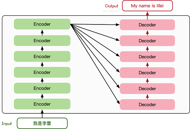
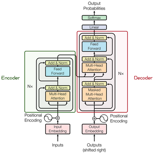
The Transformer model originated from an article in 2017 [2]. The encoder-decoder structure based on the Attention mechanism proposed in this article has achieved great success in the field of natural language processing. The model structure is shown in the figure below:
Its main structure is composed of multiple Encoder and Decoder modules, and the detailed structure of Encoder and Decoder is shown in the following figure [2]:
Encoder and Decoder consist of many structures, such as: Multi-Head Attention layer, Feed
Forward layer, Normaliztion layer, and even Residual Connection (
"Add" in the figure). However, the most important structure is the Multi-Head Attention
structure, which is based on the Self-Attention mechanism and is a parallel composition of multiple Self-Attentions.Therefore, understanding Self-Attention grasps the core of Transformer.
Attention module
from mindspore import nn, ops


class Attention(nn.Cell):
    def __init__(self,
                 dim: int,
                 num_heads: int = 8,
                 keep_prob: float = 1.0,
                 attention_keep_prob: float = 1.0):
        super(Attention, self).__init__()

        self.num_heads = num_heads
        head_dim = dim // num_heads
        self.scale = ms.Tensor(head_dim ** -0.5)

        self.qkv = nn.Dense(dim, dim * 3)
        self.attn_drop = nn.Dropout(p=1.0-attention_keep_prob)
        self.out = nn.Dense(dim, dim)
        self.out_drop = nn.Dropout(p=1.0-keep_prob)
        self.attn_matmul_v = ops.BatchMatMul()
        self.q_matmul_k = ops.BatchMatMul(transpose_b=True)
        self.softmax = nn.Softmax(axis=-1)

    def construct(self, x):
        """Attention construct."""
        b, n, c = x.shape
        qkv = self.qkv(x)
        qkv = ops.reshape(qkv, (b, n, 3, self.num_heads, c // self.num_heads))
        qkv = ops.transpose(qkv, (2, 0, 3, 1, 4))
        q, k, v = ops.unstack(qkv, axis=0)
        attn = self.q_matmul_k(q, k)
        attn = ops.mul(attn, self.scale)
        attn = self.softmax(attn)
        attn = self.attn_drop(attn)
        out = self.attn_matmul_v(attn, v)
        out = ops.transpose(out, (0, 2, 1, 3))
        out = ops.reshape(out, (b, n, c))
        out = self.out(out)
        out = self.out_drop(out)

        return out

Transformer Encoder
After understanding the Self-Attention structure, the
basic structure of Transformer can be formed by splicing with Feed Forward, Residual Connection and other structures. The following code implements the Feed Forward and Residual
Connection structure.
from typing import Optional, Dict


class FeedForward(nn.Cell):
    def __init__(self,
                 in_features: int,
                 hidden_features: Optional[int] = None,
                 out_features: Optional[int] = None,
                 activation: nn.Cell = nn.GELU,
                 keep_prob: float = 1.0):
        super(FeedForward, self).__init__()
        out_features = out_features or in_features
        hidden_features = hidden_features or in_features
        self.dense1 = nn.Dense(in_features, hidden_features)
        self.activation = activation()
        self.dense2 = nn.Dense(hidden_features, out_features)
        self.dropout = nn.Dropout(p=1.0-keep_prob)

    def construct(self, x):
        """Feed Forward construct."""
        x = self.dense1(x)
        x = self.activation(x)
        x = self.dropout(x)
        x = self.dense2(x)
        x = self.dropout(x)

        return x


class ResidualCell(nn.Cell):
    def __init__(self, cell):
        super(ResidualCell, self).__init__()
        self.cell = cell

    def construct(self, x):
        """ResidualCell construct."""
        return self.cell(x) + x

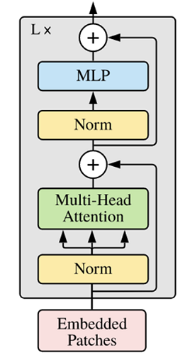
Next, use Self-Attention to build the TransformerEncoder part of the ViT model, which is similar to building a Transformer encoder part, as shown in the following figure [1]:
vit-encoder
The basic structure in the ViT model is different from the standard Transformer, mainly because the position of Normalization is placed before Self-Attention and Feed
Forward, and other structures such as Residual Connection, Feed
Forward, and Normalization are designed as in Transformer.From the picture of the Transformer structure, it can be found that the stacking of multiple sub-encoders completes the construction of the model encoder. In the ViT model, this idea is still followed. By configuring the hyperparameter num_layers, the number of stacked layers can be determined.
The structure of Residual
Connection and Normalization can ensure the strong scalability of the model (to ensure that the information will not degrade after deep processing, which is the role of Residual
Connection), and the application of Normalization and dropout can enhance the generalization ability of the model.The structure of Transformer can be clearly seen from the following source code. Combining the TransformerEncoder structure with a multi-layer perceptron (MLP) constitutes the backbone part of the ViT model.
class TransformerEncoder(nn.Cell):
    def __init__(self,
                 dim: int,
                 num_layers: int,
                 num_heads: int,
                 mlp_dim: int,
                 keep_prob: float = 1.,
                 attention_keep_prob: float = 1.0,
                 drop_path_keep_prob: float = 1.0,
                 activation: nn.Cell = nn.GELU,
                 norm: nn.Cell = nn.LayerNorm):
        super(TransformerEncoder, self).__init__()
        layers = []

        for _ in range(num_layers):
            normalization1 = norm((dim,))
            normalization2 = norm((dim,))
            attention = Attention(dim=dim,
                                  num_heads=num_heads,
                                  keep_prob=keep_prob,
                                  attention_keep_prob=attention_keep_prob)

            feedforward = FeedForward(in_features=dim,
                                      hidden_features=mlp_dim,
                                      activation=activation,
                                      keep_prob=keep_prob)

            layers.append(
                nn.SequentialCell([
                    ResidualCell(nn.SequentialCell([normalization1, attention])),
                    ResidualCell(nn.SequentialCell([normalization2, feedforward]))
                ])
            )
        self.layers = nn.SequentialCell(layers)

    def construct(self, x):
        """Transformer construct."""
        return self.layers(x)

Input of ViT model
The traditional Transformer structure is mainly used to process word vectors (Word Embedding or Word Vector) in the field of natural language. The main difference between word vectors and traditional image data is that word vectors are usually stacked as one-dimensional vectors, while pictures are two-dimensional matrices Stacking, the multi-head attention mechanism will extract the connection between word vectors when processing the stacking of one-dimensional word vectors, that is, the context semantics, which makes Transformer very useful in the field of natural language processing, and how does the two-dimensional image matrix compare with one-dimensional Word vector conversion has become a small threshold for Transformer to enter the field of image processing.
In the ViT model:
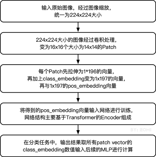
By dividing the input image into 16*16 patches on each channel, this step is done through a convolution operation. Of course, it can also be divided manually, but the convolution operation can also achieve the purpose and can be performed once. Data processing; for example, an input
image of 224 x 224 is first processed by convolution to obtain 16 x 16 patches, then the size of each patch is 14 x 14.
Then stretch the matrix of each patch into a one-dimensional vector, thus obtaining the effect of approximate word vector stacking. The 14 x 14 patch obtained in the previous step is converted into a vector of length 196.
This is the first step through which the image input network goes through. The specific Patch Embedding code is as follows:
class PatchEmbedding(nn.Cell):
    MIN_NUM_PATCHES = 4

    def __init__(self,
                 image_size: int = 224,
                 patch_size: int = 16,
                 embed_dim: int = 768,
                 input_channels: int = 3):
        super(PatchEmbedding, self).__init__()

        self.image_size = image_size
        self.patch_size = patch_size
        self.num_patches = (image_size // patch_size) ** 2
        self.conv = nn.Conv2d(input_channels, embed_dim, kernel_size=patch_size, stride=patch_size, has_bias=True)

    def construct(self, x):
        """Path Embedding construct."""
        x = self.conv(x)
        b, c, h, w = x.shape
        x = ops.reshape(x, (b, c, h * w))
        x = ops.transpose(x, (0, 2, 1))

        return x

After the input image is divided into patches, it will go through two processes of pos_embedding and class_embedding.
class_embedding mainly draws on the idea of the BERT model for text classification, adding a category value before each word
vector, usually at the first place in the vector, and adding class_embedding to the 196-dimensional vector obtained in the previous step becomes 197 dimensions.The added class_embedding is a parameter that can be learned. After continuous training of the network, the final output category is finally determined by the output of the first dimension of the output vector; since the input is 16 x 16 patches, the output is classified as 16 x 16 class_embeddings for classification.
pos_embedding is also a set of learnable parameters that will be added to the processed patch matrix.
Since pos_embedding is also a learnable parameter, its addition is similar to the bias of the full link network and convolution. This step is to create a trainable vector with a length dimension of 197 and add it to the vector after class_embedding.
In fact, pos_embedding has 4 schemes in total. However, after the author's argument, only adding pos_embedding and not adding pos_embedding has a significant impact. As for whether pos_embedding is one-dimensional or two-dimensional, it has little effect on the classification results. Therefore, in our code, one-dimensional pos_embedding is also used. Because class_embedding is added before pos_embedding, so the dimension of pos_embedding will be 1 higher than the dimension after patch stretching.
In general, the ViT model still takes advantage of the Transformer model in dealing with contextual semantics, and converts the image into a "variant word vector" and then processes it. The significance of this conversion is that there is space between multiple patches. Contact, which is similar to a kind of "spatial semantics", thus obtaining a better processing effect.
Build ViT as a whole
The following code builds a complete ViT model.
from mindspore.common.initializer import Normal
from mindspore.common.initializer import initializer
from mindspore import Parameter


def init(init_type, shape, dtype, name, requires_grad):
    """Init."""
    initial = initializer(init_type, shape, dtype).init_data()
    return Parameter(initial, name=name, requires_grad=requires_grad)


class ViT(nn.Cell):
    def __init__(self,
                 image_size: int = 224,
                 input_channels: int = 3,
                 patch_size: int = 16,
                 embed_dim: int = 768,
                 num_layers: int = 12,
                 num_heads: int = 12,
                 mlp_dim: int = 3072,
                 keep_prob: float = 1.0,
                 attention_keep_prob: float = 1.0,
                 drop_path_keep_prob: float = 1.0,
                 activation: nn.Cell = nn.GELU,
                 norm: Optional[nn.Cell] = nn.LayerNorm,
                 pool: str = 'cls') -> None:
        super(ViT, self).__init__()

        self.patch_embedding = PatchEmbedding(image_size=image_size,
                                              patch_size=patch_size,
                                              embed_dim=embed_dim,
                                              input_channels=input_channels)
        num_patches = self.patch_embedding.num_patches

        self.cls_token = init(init_type=Normal(sigma=1.0),
                              shape=(1, 1, embed_dim),
                              dtype=ms.float32,
                              name='cls',
                              requires_grad=True)

        self.pos_embedding = init(init_type=Normal(sigma=1.0),
                                  shape=(1, num_patches + 1, embed_dim),
                                  dtype=ms.float32,
                                  name='pos_embedding',
                                  requires_grad=True)

        self.pool = pool
        self.pos_dropout = nn.Dropout(p=1.0-keep_prob)
        self.norm = norm((embed_dim,))
        self.transformer = TransformerEncoder(dim=embed_dim,
                                              num_layers=num_layers,
                                              num_heads=num_heads,
                                              mlp_dim=mlp_dim,
                                              keep_prob=keep_prob,
                                              attention_keep_prob=attention_keep_prob,
                                              drop_path_keep_prob=drop_path_keep_prob,
                                              activation=activation,
                                              norm=norm)
        self.dropout = nn.Dropout(p=1.0-keep_prob)
        self.dense = nn.Dense(embed_dim, num_classes)

    def construct(self, x):
        """ViT construct."""
        x = self.patch_embedding(x)
        cls_tokens = ops.tile(self.cls_token.astype(x.dtype), (x.shape[0], 1, 1))
        x = ops.concat((cls_tokens, x), axis=1)
        x += self.pos_embedding

        x = self.pos_dropout(x)
        x = self.transformer(x)
        x = self.norm(x)
        x = x[:, 0]
        if self.training:
            x = self.dropout(x)
        x = self.dense(x)

        return x

The overall flow chart is as follows:
4. Model Training and Inference
model training
from mindspore.nn import LossBase
from mindspore.train import LossMonitor, TimeMonitor, CheckpointConfig, ModelCheckpoint
from mindspore import train

# define super parameter
epoch_size = 10
momentum = 0.9
num_classes = 1000
resize = 224
step_size = dataset_train.get_dataset_size()

# construct model
network = ViT()

# load ckpt
vit_url = "https://download.mindspore.cn/vision/classification/vit_b_16_224.ckpt"
path = "./ckpt/vit_b_16_224.ckpt"

vit_path = download(vit_url, path, replace=True)
param_dict = ms.load_checkpoint(vit_path)
ms.load_param_into_net(network, param_dict)

# define learning rate
lr = nn.cosine_decay_lr(min_lr=float(0),
                        max_lr=0.00005,
                        total_step=epoch_size * step_size,
                        step_per_epoch=step_size,
                        decay_epoch=10)

# define optimizer
network_opt = nn.Adam(network.trainable_params(), lr, momentum)


# define loss function
class CrossEntropySmooth(LossBase):
    """CrossEntropy."""

    def __init__(self, sparse=True, reduction='mean', smooth_factor=0., num_classes=1000):
        super(CrossEntropySmooth, self).__init__()
        self.onehot = ops.OneHot()
        self.sparse = sparse
        self.on_value = ms.Tensor(1.0 - smooth_factor, ms.float32)
        self.off_value = ms.Tensor(1.0 * smooth_factor / (num_classes - 1), ms.float32)
        self.ce = nn.SoftmaxCrossEntropyWithLogits(reduction=reduction)

    def construct(self, logit, label):
        if self.sparse:
            label = self.onehot(label, ops.shape(logit)[1], self.on_value, self.off_value)
        loss = self.ce(logit, label)
        return loss


network_loss = CrossEntropySmooth(sparse=True,
                                  reduction="mean",
                                  smooth_factor=0.1,
                                  num_classes=num_classes)

# set checkpoint
ckpt_config = CheckpointConfig(save_checkpoint_steps=step_size, keep_checkpoint_max=100)
ckpt_callback = ModelCheckpoint(prefix='vit_b_16', directory='./ViT', config=ckpt_config)

# initialize model
# "Ascend + mixed precision" can improve performance
ascend_target = (ms.get_context("device_target") == "Ascend")
if ascend_target:
    model = train.Model(network, loss_fn=network_loss, optimizer=network_opt, metrics={

    "acc"}, amp_level="O2")
else:
    model = train.Model(network, loss_fn=network_loss, optimizer=network_opt, metrics={

    "acc"}, amp_level="O0")

# train model
model.train(epoch_size,
            dataset_train,
            callbacks=[ckpt_callback, LossMonitor(125), TimeMonitor(125)],
            dataset_sink_mode=False,)

model validation
dataset_val = ImageFolderDataset(os.path.join(data_path, "val"), shuffle=True)

trans_val = [
    transforms.Decode(),
    transforms.Resize(224 + 32),
    transforms.CenterCrop(224),
    transforms.Normalize(mean=mean, std=std),
    transforms.HWC2CHW()
]

dataset_val = dataset_val.map(operations=trans_val, input_columns=["image"])
dataset_val = dataset_val.batch(batch_size=16, drop_remainder=True)

# construct model
network = ViT()

# load ckpt
param_dict = ms.load_checkpoint(vit_path)
ms.load_param_into_net(network, param_dict)

network_loss = CrossEntropySmooth(sparse=True,
                                  reduction="mean",
                                  smooth_factor=0.1,
                                  num_classes=num_classes)

# define metric
eval_metrics = {

    'Top_1_Accuracy': train.Top1CategoricalAccuracy(),
                'Top_5_Accuracy': train.Top5CategoricalAccuracy()}

if ascend_target:
    model = train.Model(network, loss_fn=network_loss, optimizer=network_opt, metrics=eval_metrics, amp_level="O2")
else:
    model = train.Model(network, loss_fn=network_loss, optimizer=network_opt, metrics=eval_metrics, amp_level="O0")

# evaluate model
result = model.eval(dataset_val)
print(result)

model reasoning
dataset_infer = ImageFolderDataset(os.path.join(data_path, "infer"), shuffle=True)

trans_infer = [
    transforms.Decode(),
    transforms.Resize([224, 224]),
    transforms.Normalize(mean=mean, std=std),
    transforms.HWC2CHW()
]

dataset_infer = dataset_infer.map(operations=trans_infer,
                                  input_columns=["image"],
                                  num_parallel_workers=1)
dataset_infer = dataset_infer.batch(1)
import os
import pathlib
import cv2
import numpy as np
from PIL import Image
from enum import Enum
from scipy import io
class Color(Enum):
"""dedine enum color."""
red = (0, 0, 255)
green = (0, 255, 0)
blue = (255, 0, 0)
cyan = (255, 255, 0)
yellow = (0, 255, 255)
magenta = (255, 0, 255)
white = (255, 255, 255)
black = (0, 0, 0)
def check_file_exist(file_name: str):
"""check_file_exist."""
if not os.path.isfile(file_name):
raise FileNotFoundError(f"File `{
file_name}` does not exist.")
def color_val(color):
"""color_val."""
if isinstance(color, str):
return Color[color].value
if isinstance(color, Color):
return color.value
if isinstance(color, tuple):
assert len(color) == 3
for channel in color:
assert 0 <= channel <= 255
return color
if isinstance(color, int):
assert 0 <= color <= 255
return color, color, color
if isinstance(color, np.ndarray):
assert color.ndim == 1 and color.size == 3
assert np.all((color >= 0) & (color <= 255))
color = color.astype(np.uint8)
return tuple(color)
raise TypeError(f'Invalid type for color: {type(color)}')
def imread(image, mode=None):
"""imread."""
if isinstance(image, pathlib.Path):
image = str(image)
if isinstance(image, np.ndarray):
pass
elif isinstance(image, str):
check_file_exist(image)
image = Image.open(image)
if mode:
image = np.array(image.convert(mode))
else:
raise TypeError("Image must be a `ndarray`, `str` or Path object.")
return image
def imwrite(image, image_path, auto_mkdir=True):
"""imwrite."""
if auto_mkdir:
dir_name = os.path.abspath(os.path.dirname(image_path))
if dir_name != '':
dir_name = os.path.expanduser(dir_name)
os.makedirs(dir_name, mode=777, exist_ok=True)
image = Image.fromarray(image)
image.save(image_path)
def imshow(img, win_name='', wait_time=0):
"""imshow"""
cv2.imshow(win_name, imread(img))
if wait_time == 0: # prevent from hanging if windows was closed
while True:
ret = cv2.waitKey(1)
closed = cv2.getWindowProperty(win_name, cv2.WND_PROP_VISIBLE) < 1
# if user closed window or if some key pressed
if closed or ret != -1:
break
else:
ret = cv2.waitKey(wait_time)
def show_result(img: str,
result: Dict[int, float],
text_color: str = 'green',
font_scale: float = 0.5,
row_width: int = 20,
show: bool = False,
win_name: str = '',
wait_time: int = 0,
out_file: Optional[str] = None) -> None:
"""Mark the prediction results on the picture."""
img = imread(img, mode="RGB")
img = img.copy()
x, y = 0, row_width
text_color = color_val(text_color)
for k, v in result.items():
if isinstance(v, float):
v = f'{v:.2f}'
label_text = f'{k}: {v}'
cv2.putText(img, label_text, (x, y), cv2.FONT_HERSHEY_COMPLEX,
font_scale, text_color)
y += row_width
if out_file:
show = False
imwrite(img, out_file)
if show:
imshow(img, win_name, wait_time)
def index2label():
"""Dictionary output for image numbers and categories of the ImageNet dataset."""
metafile = os.path.join(data_path, "ILSVRC2012_devkit_t12/data/meta.mat")
meta = io.loadmat(metafile, squeeze_me=True)['synsets']
nums_children = list(zip(*meta))[4]
meta = [meta[idx] for idx, num_children in enumerate(nums_children) if num_children == 0]
_, wnids, classes = list(zip(*meta))[:3]
clssname = [tuple(clss.split(', ')) for clss in classes]
wnid2class = {
wnid: clss for wnid, clss in zip(wnids, clssname)}
wind2class_name = sorted(wnid2class.items(), key=lambda x: x[0])
mapping = {
}
for index, (_, class_name) in enumerate(wind2class_name):
mapping[index] = class_name[0]
return mapping
# Read data for inference
for i, image in enumerate(dataset_infer.create_dict_iterator(output_numpy=True)):
image = image["image"]
image = ms.Tensor(image)
prob = model.predict(image)
label = np.argmax(prob.asnumpy(), axis=1)
mapping = index2label()
output = {
int(label): mapping[int(label)]}
print(output)
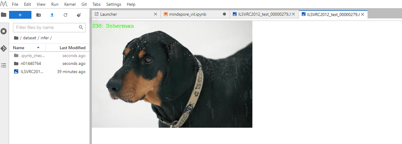
show_result(img="./dataset/infer/n01440764/ILSVRC2012_test_00000279.JPEG",
result=output,
out_file="./dataset/infer/ILSVRC2012_test_00000279.JPEG")

After the inference process is completed, you can find the inference result of the picture under the inference folder. It can be seen that the prediction result is Doberman, which is the same as the expected result, which verifies the accuracy of the model.