Deep Learning Application - Computer Vision - Image Classification [3]: Detailed introduction to model structure, implementation, and model features of ResNeXt, Res2Net, Swin Transformer, Vision Transformer, etc.

[Introduction to advanced deep learning] must-see series, including activation function, optimization strategy, loss function, model tuning, normalization algorithm, convolution model, sequence model, pre-training model, adversarial neural network, etc.

The column introduces in detail: [Introduction to advanced deep learning] must-see series, including activation function, optimization strategy, loss function, model tuning, normalization algorithm, convolution model, sequence model, pre-training model, adversarial neural network, etc.

This column is mainly to facilitate beginners to quickly grasp relevant knowledge. In the follow-up, we will continue to analyze the knowledge principles involved in deep learning to everyone, so that everyone can reserve knowledge while practicing the project, knowing what it is, why it is, and why to know why it is.

Disclaimer: Some projects are online classic projects for everyone to learn quickly, and practical links will be added in the future (competitions, papers, practical applications, etc.)

Column subscription:

• Introductory to advanced column of deep learning
• Practical articles on deep learning application projects

Deep Learning Application - Computer Vision - Image Classification [3]: Detailed introduction to model structure, implementation, and model features of ResNeXt, Res2Net, Swin Transformer, Vision Transformer, etc.

1.ResNet

Compared with VGG's 19 layers and GoogLeNet's 22 layers, ResNet can provide 18, 34, 50, 101, 152 or even more layers of networks while achieving better accuracy. But why use a deeper network? At the same time, if it's just a stack of network layers, why didn't the predecessors achieve the same success as ResNet?

1.1. A deeper network?

In theory, deepening deep learning networks can improve performance. The deep network integrates low/medium/high-level features and classifiers in an end-to-end multi-layer manner, and the level of features can be enriched by deepening the network level. To give an example, when the deep learning network has only one layer, the features to be learned will be very complex, but if there are multiple layers, it can be learned layer by layer, as shown in Figure layer of the network learns edges and colors , the second layer has learned the texture, the third layer has learned the local shape, and the fifth layer has gradually learned the global feature. The deepening of the network can theoretically provide better expression ability, so that each layer can learn more detailed features.

1.2. Why is a deep network not just a stack of layers?

1.2.1 Gradient disappears or explodes

But is network deepening really as simple as stacking layers? of course not! First, the most obvious problem is vanishing/exploding gradients. We all know that the parameter update of the neural network relies on gradient backpropagation (Back Propagation), so why do gradients disappear and explode? Give an example to explain. As shown in Figure 2, assuming that there is only one neuron in each layer, and the activation function uses the Sigmoid function, there are:

$$\begin{gathered} z_{i+1}=w_i{a}_i+b_i \\ {a}_{i+1}=s(z_{i+1}) \end{gathered}$$

where $\sigma (\cdot )$ is the sigmoid function.

According to chain derivation and backpropagation, we can get:

$$\begin{gathered} \frac{\partial y}{\partial a_1}=\frac{\partial y}{\partial a_4}\frac{\partial a_4}{\partial z_4}\frac{\partial z_4}{\partial a_3}\frac{\partial a_3}{\partial z_3}\frac{\partial z_3}{\partial a_2}\frac{\partial a_2}{\partial z_2}\frac{\partial z_2}{\partial a_1} \\ =\frac{\partial y}{\partial a_4}{p}^{{}^{\prime }}(z_4)w_3{p}^{{}^{\prime }}\left(z_3\right)w_2{p}^{{}^{\prime }}\left(z_2\right)w_1 \end{gathered}$$
The derivative of the Sigmoid function $p^{{}^{\prime }}\left(x\right)$as shown in Figure:

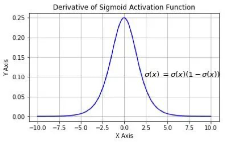
We can see that the maximum value of the derivative of sigmoid is 0.25, then as the number of network layers increases, the constant multiplication of decimals less than 1 leads to $\frac{\partial y}{\partial a_1}$Gradually approaching zero, resulting in vanishing gradient.

So how did the gradient explosion cause it? In the same way, when the weight is initialized to a large value, although multiplying it with the derivative of the activation function will reduce this value, but as the neural network deepens, the gradient increases exponentially, which will cause a gradient explosion. But since AlexNet, the ReLU function has been used to replace Sigmoid in the neural network, and the addition of the BN (Batch Normalization) layer has basically solved the problem of gradient disappearance/explosion.

1.2.2 Network degradation

Now that the problem of gradient disappearance/explosion is solved, can the network be deepened by stacking layers? Still no!

Let's take a look at the example mentioned in the ResNet paper (see Figure 4). It is obvious that the performance of the 56-layer deep network on the training set and the test set is far inferior to the 20-layer shallow network. As the number of layers deepens, the accuracy gradually saturates, and then drops sharply. The specific performance is that the training effect of the deep network is not as good as that of the shallow network, which is called network degradation.

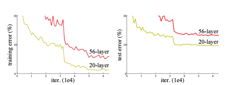
Why does it cause network degradation? According to the theoretical idea, when the effect of the shallow network is good, the increase in the number of network layers should not make the effect of the model worse even if it does not lead to an improvement in accuracy. But in fact, the existence of nonlinear activation functions will cause a lot of irreversible information loss. When the network deepens to a certain extent, excessive information loss will cause network degradation.

And ResNet is to propose a method to allow the network to have the same mapping ability, that is, as the number of network layers increases, the deep network will at least not be worse than the shallow network.

1…3. Residual block

Now we understand that in order to deepen the network structure and learn more detailed features each time to improve network accuracy, one thing that needs to be implemented is identity mapping . So how can residual networks do this?

The identity map is $H(x)=x$ , the existing neural network structure is difficult to do this, but if we design the network as$H\left(x\right)=F(x)+x$，即 $F\left(x\right)=H\left(x\right)-x$ , then only need to make the residual function$F\left(x\right)=0$ , constitutes the identity map$H\left(x\right)=F(x)$。

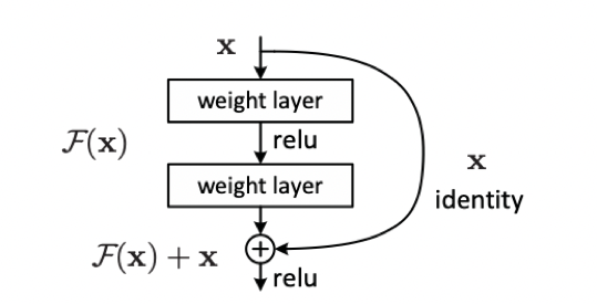
The purpose of the residual structure is to make F ( x ) F(x) as the network deepens$F\left(x\right)$ is close to 0, so that the accuracy of the deep network will not drop based on the optimal shallow network. Seeing this, you may have doubts. In this case, why not directly select the optimal shallow network? This is because the optimal shallow network structure is not easy to find, and ResNet can find the optimal shallow network by increasing the depth and ensure that the deep network will not degrade due to the superposition of layers.

• references

[1] Visualizing and Understanding Convolutional Networks

[2] Deep Residual Learning for Image Recognition

2. ResNeXt（2017）

ResNeXt is a new image classification network proposed by He Kaiming's team at the 2017 CVPR conference. ResNeXt is an upgraded version of ResNet. On the basis of ResNet, the concept of cardinality is introduced. Similar to ResNet, ResNeXt also has ResNeXt-50 and ResNeXt-101 versions. So compared to ResNet, where is the innovation of ResNeXt? Since it is a classification network, how have the indicators on the ImageNet dataset changed compared to ResNet? What is ResNeXt_WSL after? Let me share this knowledge with you.

2.1 ResNeXt model structure

In the ResNeXt paper, the author raised a common problem at that time. If the accuracy of the model is to be improved, the method of deepening the network or widening the network is often adopted. Although this method is effective, it comes with the difficulty of network design and the increase of computational overhead. It is often necessary to pay a greater price for a little improvement in accuracy. Therefore, a better strategy is needed to improve the accuracy of the network without additional computational cost. Thus, who proposed the concept of cardinality.

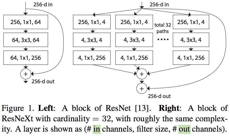
The figure below shows the difference between ResNet (left) and ResNeXt (right) blocks. In ResNet, the input feature with 256 channels is compressed by 4 times to 64 channels through 1×1 convolution, and then the 3×3 convolution kernel is used to process the features, and the number of channels is expanded by 1×1 convolution to be the same as the original Output after feature residual connection. ResNeXt is also the same processing strategy, but in ResNeXt, the input features with 256 channels are divided into 32 groups, and each group is compressed 64 times to 4 channels for processing. The 32 groups are added and connected with the original feature residuals to output. Here cardinatity refers to the number of identical branches in a block.

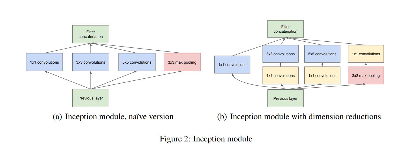
The figure below shows the two inception module structures of InceptionNet. The left side is the naive version of the inception module, and the right side is the inception module using the dimensionality reduction method. Compared with the right side, the obvious disadvantage of the left side is that the parameters are large and the amount of calculation is huge. The purpose of using convolution kernels of different sizes is to extract feature information of different scales. For images, multi-scale information helps the network to better select image information, and makes the network more effective for image inputs of different sizes. Good adaptability, but the problem brought by multi-scale is the increase in the amount of calculation. Therefore, in the model on the right, InceptionNet solves this problem very well. First, the convolution of 1×1 is used for feature dimensionality reduction. After reducing the number of feature channels, a multi-scale structure is used to extract feature information. After reducing the parameters Quantitatively capture multi-scale feature information at the same time.

ResNeXt draws on this "segmentation-transformation-aggregation" strategy, but uses the same topology to build ResNeXt modules. Each structure is the same convolution kernel, which keeps the structure simple and makes the model more convenient and easier to program, while InceptionNet requires a more complex design.

2.2 ResNeXt model implementation

The model structure of ResNeXt is consistent with that of ResNet, the main difference lies in the construction of the block, so here we use the paddle framework to implement the code of the block

class ConvBNLayer(nn.Layer):
    def __init__(self, num_channels, num_filters, filter_size, stride=1,
                 groups=1, act=None, name=None, data_format="NCHW"
                ):
        super(ConvBNLayer, self).__init__()
        self._conv = Conv2D(
            in_channels=num_channels, out_channels=num_filters,
            kernel_size=filter_size, stride=stride,
            padding=(filter_size - 1) // 2, groups=groups,
            weight_attr=ParamAttr(name=name + "_weights"), bias_attr=False,
            data_format=data_format
        )
        if name == "conv1":
            bn_name = "bn_" + name
        else:
            bn_name = "bn" + name[3:]
        self._batch_norm = BatchNorm(
            num_filters, act=act, param_attr=ParamAttr(name=bn_name + '_scale'),
            bias_attr=ParamAttr(bn_name + '_offset'), moving_mean_name=bn_name + '_mean',
            moving_variance_name=bn_name + '_variance', data_layout=data_format
        )

    def forward(self, inputs):
        y = self._conv(inputs)
        y = self._batch_norm(y)
        return y


class BottleneckBlock(nn.Layer):
    def __init__(self, num_channels, num_filters, stride, cardinality, shortcut=True,
                 name=None, data_format="NCHW"
                ):
        super(BottleneckBlock, self).__init__()
        self.conv0 = ConvBNLayer(num_channels=num_channels, num_filters=num_filters,
            filter_size=1, act='relu', name=name + "_branch2a",
            data_format=data_format
           )
        self.conv1 = ConvBNLayer(
            num_channels=num_filters, num_filters=num_filters,
            filter_size=3, groups=cardinality,
            stride=stride, act='relu', name=name + "_branch2b",
            data_format=data_format
        )

        self.conv2 = ConvBNLayer(
            num_channels=num_filters,
            num_filters=num_filters * 2 if cardinality == 32 else num_filters,
            filter_size=1, act=None,
            name=name + "_branch2c",
            data_format=data_format
        )

        if not shortcut:
            self.short = ConvBNLayer(
                num_channels=num_channels, num_filters=num_filters * 2
                if cardinality == 32 else num_filters,
                filter_size=1, stride=stride,
                name=name + "_branch1", data_format=data_format
            )

        self.shortcut = shortcut

    def forward(self, inputs):
        y = self.conv0(inputs)
        conv1 = self.conv1(y)
        conv2 = self.conv2(conv1)

        if self.shortcut:
            short = inputs
        else:
            short = self.short(inputs)

        y = paddle.add(x=short, y=conv2)
        y = F.relu(y)
        return y

2.3 ResNeXt model features

1. By controlling the number of cardinality, ResNeXt makes the parameters and GFLOPs of ResNeXt almost the same as ResNet.
2. Through the branch structure of cardinality, more nonlinearity is provided for the network, so as to obtain more accurate classification effect.

2.4 ResNeXt model indicators

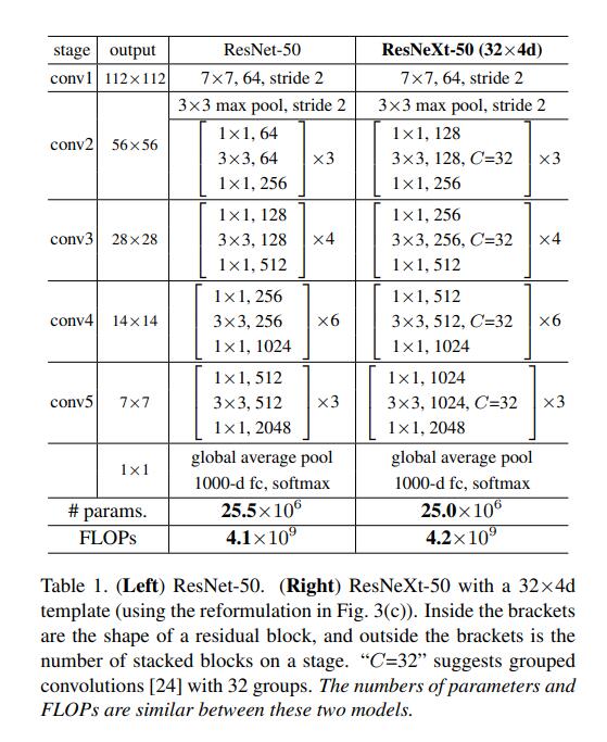
The above figure is a comparison of the parameters of ResNet and ResNeXt. It can be seen that ResNeXt and ResNet have almost the same amount of parameters and calculations, but the performance of the two on ImageNet is different.

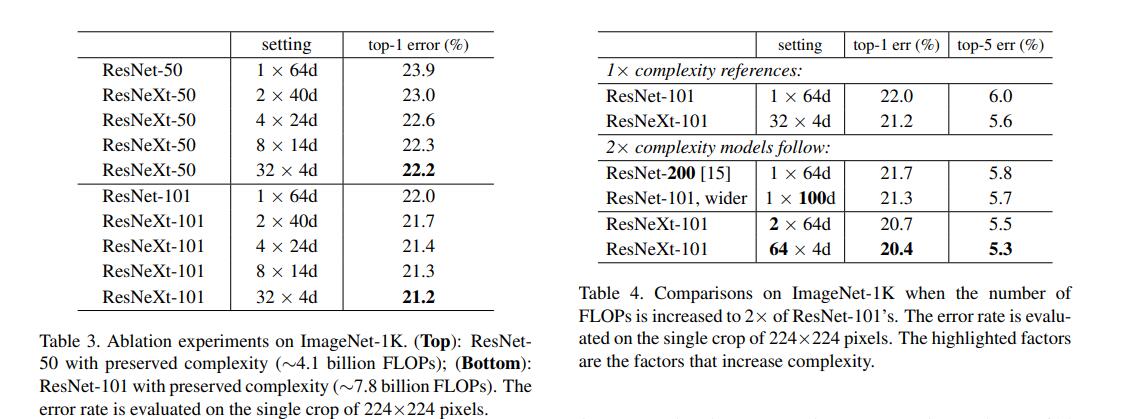
It can be seen from the figure that in addition to increasing the number of channels of the 3×3 convolution kernel in the block, ResNeXt can also increase the number of branches of cardinality to improve the accuracy of the model. Both ResNeXt-50 and ResNeXt-101 greatly reduce the error rate corresponding to ResNet. In the figure, ResNeXt-101 changes from 32×4d to 64×4d. Although the amount of calculation is doubled, it can also effectively reduce the classification error rate.

In 2019, He Kaiming's team opened up ResNeXt_WSL. ResNeXt_WSL is the ResNeXt trained by He Kaiming's team using weakly supervised learning. The WSL in ResNeXt_WSL means Weakly Supervised Learning (weakly supervised learning).

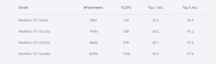
ResNeXt101_32×48d_WSL has 800 million+ parameters. It is trained on the Instagram dataset through weakly supervised learning pre-training method, and then fine-tuned with the ImageNet dataset. Instagram has 940 million pictures, which have not been specially marked, only with Hashtags added by users themselves.
ResNeXt_WSL has the same structure as ResNeXt, but the training method has changed. The figure below is the training effect of ResNeXt_WSL.

• 6. ReferencesResNet
     _

ResNeXt

GoogLeNet

3.Res2Net（2020）

In 2020, Cheng Mingming Group of Nankai University proposed a new module Res2Net for target detection tasks. And his paper has been accepted by TPAMI2020. Res2Net, like ResNeXt, is a variant of ResNet, but Res2Net not only improves the accuracy of classification tasks, but also improves the accuracy of detection tasks. The new module of Res2Net can be easily integrated with other existing excellent modules. Without increasing the computational load, the test performance on ImageNet, CIFAR-100 and other data sets exceeds ResNet. Because there are residual connections in the residual block of the model, it is named Res2Net.

3.1 Res2Net model structure

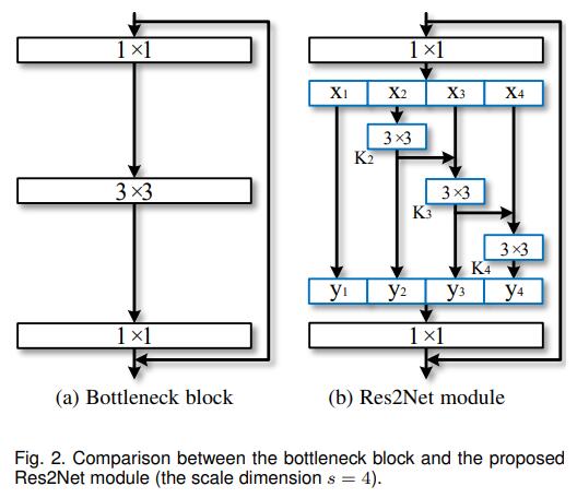
The model structure looks very simple. The input feature x is split into k features, and the i+1th (i = 0, 1, 2,...,k-1) feature is convolved with a residual of 3×3 The way of connection is fused into the i+2th feature. This is the main structure of Res2Net. So what is the purpose of doing this? What good can it do?
The answer is multi-scale convolution. Multi-scale features have always been very important in detection tasks. Since the introduction of hole convolution, the multi-scale pyramid model based on hole convolution has achieved milestone results in detection tasks. The information of objects obtained under different receptive fields is different. Small receptive fields may see more details of objects, which is also of great benefit for detecting small targets, while large receptive fields can feel the overall structure of objects, which is convenient The network locates the position of the object, and the combination of details and position can better obtain object information with clear boundaries. Therefore, models combined with multi-scale pyramids can often achieve good results. In Res2Net, the feature k2 is sent to the processing flow where x3 is located after 3×3 convolution, k2 is again optimized by 3×3 convolution, and two 3×3 convolutions are equivalent to a 5×5 convolution. Then, k3 takes it for granted and combines the processed features of the 3×3 receptive field and the 5×5 receptive field. By analogy, the 7×7 receptive field is applied in k4. In this way, Res2Net extracts multi-scale features for detection tasks to improve the accuracy of the model. In this paper, s is the control parameter of the scale size, that is, the number of input channels can be equally divided into multiple feature channels. The larger the s, the stronger the multi-scale capability, and some additional computational overhead can also be ignored.

3.2 Res2Net model implementation

The model structure of Res2Net and ResNet is the same, the main difference lies in the construction of the block, so here we use the paddle framework to realize the code of the block

class ConvBNLayer(nn.Layer):
    def __init__(
            self,
            num_channels,
            num_filters,
            filter_size,
            stride=1,
            groups=1,
            is_vd_mode=False,
            act=None,
            name=None, ):
        super(ConvBNLayer, self).__init__()

        self.is_vd_mode = is_vd_mode
        self._pool2d_avg = AvgPool2D(
            kernel_size=2, stride=2, padding=0, ceil_mode=True)
        self._conv = Conv2D(
            in_channels=num_channels,
            out_channels=num_filters,
            kernel_size=filter_size,
            stride=stride,
            padding=(filter_size - 1) // 2,
            groups=groups,
            weight_attr=ParamAttr(name=name + "_weights"),
            bias_attr=False)
        if name == "conv1":
            bn_name = "bn_" + name
        else:
            bn_name = "bn" + name[3:]
        self._batch_norm = BatchNorm(
            num_filters,
            act=act,
            param_attr=ParamAttr(name=bn_name + '_scale'),
            bias_attr=ParamAttr(bn_name + '_offset'),
            moving_mean_name=bn_name + '_mean',
            moving_variance_name=bn_name + '_variance')

    def forward(self, inputs):
        if self.is_vd_mode:
            inputs = self._pool2d_avg(inputs)
        y = self._conv(inputs)
        y = self._batch_norm(y)
        return y


class BottleneckBlock(nn.Layer):
    def __init__(self,
                 num_channels1,
                 num_channels2,
                 num_filters,
                 stride,
                 scales,
                 shortcut=True,
                 if_first=False,
                 name=None):
        super(BottleneckBlock, self).__init__()
        self.stride = stride
        self.scales = scales
        self.conv0 = ConvBNLayer(
            num_channels=num_channels1,
            num_filters=num_filters,
            filter_size=1,
            act='relu',
            name=name + "_branch2a")
        self.conv1_list = []
        for s in range(scales - 1):
            conv1 = self.add_sublayer(
                name + '_branch2b_' + str(s + 1),
                ConvBNLayer(
                    num_channels=num_filters // scales,
                    num_filters=num_filters // scales,
                    filter_size=3,
                    stride=stride,
                    act='relu',
                    name=name + '_branch2b_' + str(s + 1)))
            self.conv1_list.append(conv1)
        self.pool2d_avg = AvgPool2D(kernel_size=3, stride=stride, padding=1)

        self.conv2 = ConvBNLayer(
            num_channels=num_filters,
            num_filters=num_channels2,
            filter_size=1,
            act=None,
            name=name + "_branch2c")

        if not shortcut:
            self.short = ConvBNLayer(
                num_channels=num_channels1,
                num_filters=num_channels2,
                filter_size=1,
                stride=1,
                is_vd_mode=False if if_first else True,
                name=name + "_branch1")

        self.shortcut = shortcut

    def forward(self, inputs):
        y = self.conv0(inputs)
        xs = paddle.split(y, self.scales, 1)
        ys = []
        for s, conv1 in enumerate(self.conv1_list):
            if s == 0 or self.stride == 2:
                ys.append(conv1(xs[s]))
            else:
                ys.append(conv1(xs[s] + ys[-1]))
        if self.stride == 1:
            ys.append(xs[-1])
        else:
            ys.append(self.pool2d_avg(xs[-1]))
        conv1 = paddle.concat(ys, axis=1)
        conv2 = self.conv2(conv1)

        if self.shortcut:
            short = inputs
        else:
            short = self.short(inputs)
        y = paddle.add(x=short, y=conv2)
        y = F.relu(y)
        return y

3.3 Model Features

1. It can be integrated with other structures, such as SENEt, ResNeXt, DLA, etc., to increase the accuracy.
2. The calculation load does not increase, and the feature extraction capability is stronger.

3.4 Model indicators

ImageNet classification effect as shown below

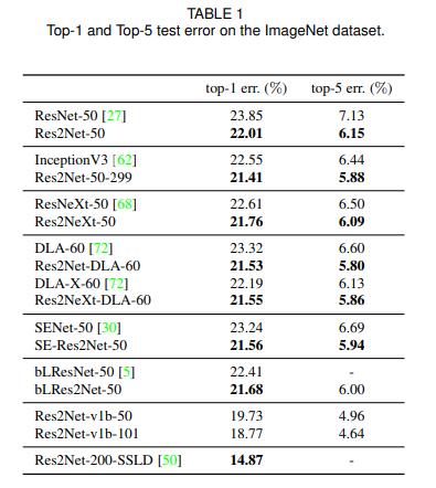
Res2Net-50 is the version that benchmarks ResNet50.

Res2Net-50-299 refers to the Res2Net-50 that cuts the input picture to 299×299 for prediction, because it is generally cut or resized to 224×224.

Res2NeXt-50 is Res2Net-50 fused with ResNeXt.

Res2Net-DLA-60 refers to Res2Net-50 fused with DLA-60.

Res2NeXt-DLA-60 is a Res2Net-50 that combines ResNeXt and DLA-60.

SE-Res2Net-50 is Res2Net-50 fused with SENet.

blRes2Net-50 is Res2Net-50 that incorporates Big-Little Net.

Res2Net-v1b-50 is Res2Net-50 that adopts the same processing method as ResNet-vd-50.

Res2Net-200-SSLD is obtained by using a simple semi-supervised label knowledge distillation (SSLD, Simple Semi-supervised Label Distillation) method for Paddle to improve the model effect.

It can be seen that Res2Net has achieved very good results.

The effect of the COCO data set is as follows

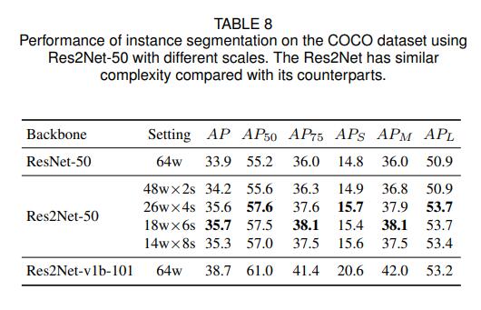
Various configurations of Res2Net-50 are higher than ResNet-50.

The effect of salient object detection dataset indicators is shown in the figure below

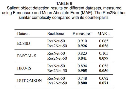
ECSSD, PASCAL-S, DUT-OMRON, and HKU-IS are the most commonly used test sets in the salient target detection task. The purpose of the salient target detection task is to segment the salient objects in the picture and represent them with white pixels. Other backgrounds Indicated by black pixels. It can be seen from the figure that using Res2Net as the backbone network has greatly improved the effect compared to ResNet.

• ReferencesRes2Net
  _

4.Swin Trasnformer（2021）

Swin Transformer is a paper published by Microsoft Research Asia this year that uses the transformer architecture to handle computer vision tasks. Swin Transformer has been slaughtered in various fields such as image classification, image segmentation, and target detection. In the paper, the author's analysis shows that there are two main reasons why Transformer has not shined in migrating from NLP to CV: 1. The two fields involved The scale is different. The token of NLP is a standard fixed size, while the feature scale of CV varies greatly. 2. CV requires a larger resolution than NLP, and the computational complexity of using Transformer in CV is the square of the image scale, which will lead to an excessively large amount of calculation. In order to solve these two problems, Swin Transformer has made two improvements compared to the previous ViT: 1. Introduce the layered construction method commonly used in CNN to build a layered Transformer 2. Introduce the idea of ​​locality, and perform self in the window area without overlap -attention calculation. In addition, Swin Transformer can be used as a general-purpose backbone network for tasks such as image classification, target detection, and semantic segmentation. It can be said that Swin Transformer may be a perfect alternative to CNN.

4.1 Swin Trasnformer model structure

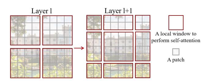
The picture below shows the comparison between Swin Transformer and ViT in processing pictures. It can be seen that Swin Transformer has the same residual structure as ResNet and the multi-scale picture structure that CNN has.

Overall summary:

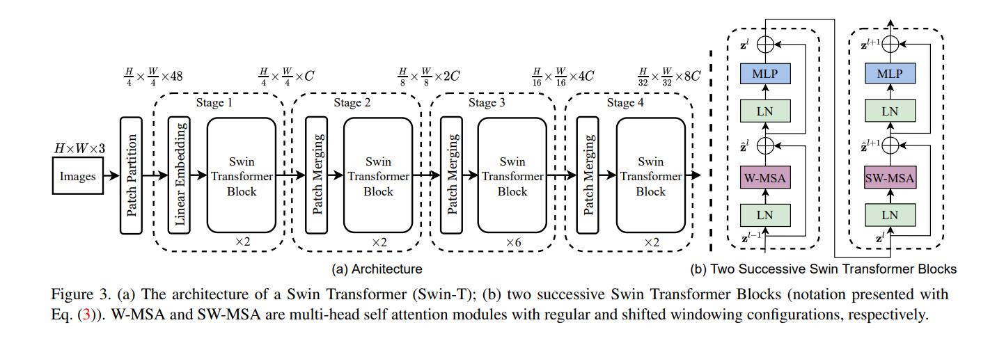
The following figure shows the network structure of Swin Transformer. The input image is first subjected to a layer of convolution for patch mapping, and the image is first divided into small blocks of 4 × 4. The image is 224 × 224 input, so there are 56 path blocks. If it is For a size of 384×384, there are 96 path blocks. Here, taking the input of 224 × 224 as an example, the input image undergoes this step, and the feature dimension of each patch is a feature map of 4x4x3=48. Therefore, the input image becomes a feature map of H/4×W/4×48. Then, the feature map starts to be input to stage1, and the linear embedding in stage1 changes the path feature dimension to C, so it becomes H/4×W/4×C. Then it is sent to the Swin Transformer Block. Before entering stage2, the Patch Merging operation is performed first. Patch Merging is very similar to the 1×1 convolution with stride=2 in CNN. Patch Merging performs downsampling before the start of each Stage, using To reduce the resolution and adjust the number of channels, when the H/4×W/4×C feature map is sent to Patch Merging, the input is merged according to 2x2 adjacent patches, so that the number of patch blocks becomes H/8 x W/8, the feature dimension becomes 4C, and then after an MLP, the feature dimension is reduced to 2C. Therefore it becomes H/8×W/8×2C. The next stage is to repeat the above process.

Each step in detail:

Linear embedding

The following uses the Paddle code to explain the architecture of the Swin Transformer step by step. The following code is the operation of Linear embedding. The whole operation can be regarded as the convolution of a patch-sized convolution kernel and a patch-sized step size to convolve the input B, C, H, and W images, and the result is naturally the size If the feature maps of B, C, H/patch, and W/patch are placed in the first Linear embedding, the resulting feature maps will be in the size of B, 96, 56, and 56. The core code of Paddle is as follows.

class PatchEmbed(nn.Layer):
    """ Image to Patch Embedding
    Args:
        img_size (int): Image size.  Default: 224.
        patch_size (int): Patch token size. Default: 4.
        in_chans (int): Number of input image channels. Default: 3.
        embed_dim (int): Number of linear projection output channels. Default: 96.
        norm_layer (nn.Layer, optional): Normalization layer. Default: None
    """

    def __init__(self,
                 img_size=224,
                 patch_size=4,
                 in_chans=3,
                 embed_dim=96,
                 norm_layer=None):
        super().__init__()
        img_size = to_2tuple(img_size)
        patch_size = to_2tuple(patch_size)
        patches_resolution = [
            img_size[0] // patch_size[0], img_size[1] // patch_size[1]
        ]
        self.img_size = img_size
        self.patch_size = patch_size
        self.patches_resolution = patches_resolution
        self.num_patches = patches_resolution[0] * patches_resolution[1] #patch个数

        self.in_chans = in_chans
        self.embed_dim = embed_dim

        self.proj = nn.Conv2D(
            in_chans, embed_dim, kernel_size=patch_size, stride=patch_size) #将stride和kernel_size设置为patch_size大小
        if norm_layer is not None:
            self.norm = norm_layer(embed_dim)
        else:
            self.norm = None

    def forward(self, x):
        B, C, H, W = x.shape
        
        x = self.proj(x) # B, 96, H/4, W4 

        x = x.flatten(2).transpose([0, 2, 1])  # B Ph*Pw 96
        if self.norm is not None:
            x = self.norm(x)
        return x

Patch Merging

The following is the operation of PatchMerging. This operation takes 2 as the step size to sample the input picture, and a total of 4 downsampled feature maps are obtained, and H and W are reduced by 2 times. Therefore, after channel-level splicing, B, 4C, H/2, W are obtained. /2 feature map. However, such splicing cannot extract useful feature information, so a linear layer filters the 4C channel to 2C, and the feature map becomes B, 2C, H/2, W/2. It can be found in detail that this operation is very similar to
the Pooling operation commonly used in convolution and the convolution operation with a step size of 2. Poling is used for downsampling, and the convolution with a step size of 2 can also be downsampled, and it also has the effect of feature screening. To sum up, after this operation, the original feature maps of B, C, H, and W become the feature maps of B, 2C, H/2, and W/2, and the downsampling operation is completed.

class PatchMerging(nn.Layer):
    r""" Patch Merging Layer.
    Args:
        input_resolution (tuple[int]): Resolution of input feature.
        dim (int): Number of input channels.
        norm_layer (nn.Layer, optional): Normalization layer.  Default: nn.LayerNorm
    """

    def __init__(self, input_resolution, dim, norm_layer=nn.LayerNorm):
        super().__init__()
        self.input_resolution = input_resolution
        self.dim = dim
        self.reduction = nn.Linear(4 * dim, 2 * dim, bias_attr=False)
        self.norm = norm_layer(4 * dim)
    
    def forward(self, x):
        """
        x: B, H*W, C
        """
        H, W = self.input_resolution
        B, L, C = x.shape
        assert L == H * W, "input feature has wrong size"
        assert H % 2 == 0 and W % 2 == 0, "x size ({}*{}) are not even.".format(
            H, W)

        x = x.reshape([B, H, W, C])
        # 每次降采样是两倍，因此在行方向和列方向上，间隔2选取元素。
        x0 = x[:, 0::2, 0::2, :]  # B H/2 W/2 C
        x1 = x[:, 1::2, 0::2, :]  # B H/2 W/2 C
        x2 = x[:, 0::2, 1::2, :]  # B H/2 W/2 C
        x3 = x[:, 1::2, 1::2, :]  # B H/2 W/2 C
        # 拼接在一起作为一整个张量，展开。通道维度会变成原先的4倍（因为H,W各缩小2倍）
        x = paddle.concat([x0, x1, x2, x3], -1)  # B H/2 W/2 4*C
        x = x.reshape([B, H * W // 4, 4 * C])  # B H/2*W/2 4*C 

        x = self.norm(x)
        # 通过一个全连接层再调整通道维度为原来的两倍
        x = self.reduction(x)

        return x

Swin Transformer Block：

The following operation is to divide the feature map according to the window_size and restore the operation. The principle is very simple, just divide it side by side.

def window_partition(x, window_size):
    """
    Args:
        x: (B, H, W, C)
        window_size (int): window size

    Returns:
        windows: (num_windows*B, window_size, window_size, C)
    """
    B, H, W, C = x.shape
    x = x.reshape([B, H // window_size, window_size, W // window_size, window_size, C])
    windows = x.transpose([0, 1, 3, 2, 4, 5]).reshape([-1, window_size, window_size, C])
    return windows


def window_reverse(windows, window_size, H, W):
    """
    Args:
        windows: (num_windows*B, window_size, window_size, C)
        window_size (int): Window size
        H (int): Height of image
        W (int): Width of image

    Returns:
        x: (B, H, W, C)
    """
    B = int(windows.shape[0] / (H * W / window_size / window_size))
    x = windows.reshape([B, H // window_size, W // window_size, window_size, window_size, -1])
    x = x.transpose([0, 1, 3, 2, 4, 5]).reshape([B, H, W, -1])
    return x

The most important thing in Swin Transformer is of course the Swin Transformer Block. Let me explain the principle of the Swin Transformer Block.
Let's take a look at MLP and LN first. MLP and LN are multi-layer perceptrons and LayerNorm relative to BatchNorm. The principle is relatively simple, so just look at the paddle code directly.

class Mlp(nn.Layer):
    def __init__(self, in_features, hidden_features=None, out_features=None, act_layer=nn.GELU, drop=0.):
        super().__init__()
        out_features = out_features or in_features
        hidden_features = hidden_features or in_features
        self.fc1 = nn.Linear(in_features, hidden_features)
        self.act = act_layer()
        self.fc2 = nn.Linear(hidden_features, out_features)
        self.drop = nn.Dropout(drop)

    def forward(self, x):
        x = self.fc1(x)
        x = self.act(x)
        x = self.drop(x)
        x = self.fc2(x)
        x = self.drop(x)
        return x

The picture below shows that the Shifted Window based MSA is the core part of Swin Transformer. Shifted Window based MSA consists of two parts, one is W-MSA (window multi-head attention), and the other is SW-MSA (shift window multi-head self-attention). These two appear together.

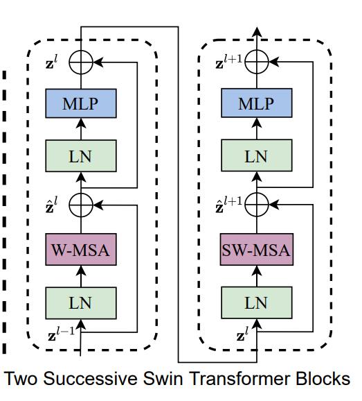
At the beginning, Swin Transformer divides a picture into 4 parts, also called 4 Windows, and then calculates the MSA of each part independently. Since each Window is independent and lacks the communication between information, the author proposes the algorithm of SW-MSA, that is, the method of using regular moving windows. Through the interaction of different windows, the exchange of characteristic information is achieved. Note that this part is the essence of this paper, students who want to understand must understand the source code

class WindowAttention(nn.Layer):
    """ Window based multi-head self attention (W-MSA) module with relative position bias.
    It supports both of shifted and non-shifted window.

    Args:
        dim (int): Number of input channels.
        window_size (tuple[int]): The height and width of the window.
        num_heads (int): Number of attention heads.
        qkv_bias (bool, optional):  If True, add a learnable bias to query, key, value. Default: True
        qk_scale (float | None, optional): Override default qk scale of head_dim ** -0.5 if set
        attn_drop (float, optional): Dropout ratio of attention weight. Default: 0.0
        proj_drop (float, optional): Dropout ratio of output. Default: 0.0
    """

    def __init__(self, dim, window_size, num_heads, qkv_bias=True, qk_scale=None, attn_drop=0., proj_drop=0.):

        super().__init__()
        self.dim = dim
        self.window_size = window_size  # Wh, Ww
        self.num_heads = num_heads
        head_dim = dim // num_heads
        self.scale = qk_scale or head_dim ** -0.5

        # define a parameter table of relative position bias
        relative_position_bias_table = self.create_parameter(
            shape=((2 * window_size[0] - 1) * (2 * window_size[1] - 1), num_heads), default_initializer=nn.initializer.Constant(value=0))  # 2*Wh-1 * 2*Ww-1, nH
        self.add_parameter("relative_position_bias_table", relative_position_bias_table)

        # get pair-wise relative position index for each token inside the window
        coords_h = paddle.arange(self.window_size[0])
        coords_w = paddle.arange(self.window_size[1])
        coords = paddle.stack(paddle.meshgrid([coords_h, coords_w]))                   # 2, Wh, Ww
        coords_flatten = paddle.flatten(coords, 1)                                     # 2, Wh*Ww
        relative_coords = coords_flatten.unsqueeze(-1) - coords_flatten.unsqueeze(1)   # 2, Wh*Ww, Wh*Ww
        relative_coords = relative_coords.transpose([1, 2, 0])                         # Wh*Ww, Wh*Ww, 2
        relative_coords[:, :, 0] += self.window_size[0] - 1                            # shift to start from 0
        relative_coords[:, :, 1] += self.window_size[1] - 1
        relative_coords[:, :, 0] *= 2 * self.window_size[1] - 1
        self.relative_position_index = relative_coords.sum(-1)                         # Wh*Ww, Wh*Ww
        self.register_buffer("relative_position_index", self.relative_position_index)

        self.qkv = nn.Linear(dim, dim * 3, bias_attr=qkv_bias)
        self.attn_drop = nn.Dropout(attn_drop)
        self.proj = nn.Linear(dim, dim)
        self.proj_drop = nn.Dropout(proj_drop)

        self.softmax = nn.Softmax(axis=-1)

    def forward(self, x, mask=None):
        """
        Args:
            x: input features with shape of (num_windows*B, N, C)
            mask: (0/-inf) mask with shape of (num_windows, Wh*Ww, Wh*Ww) or None
        """
        B_, N, C = x.shape
        qkv = self.qkv(x).reshape([B_, N, 3, self.num_heads, C // self.num_heads]).transpose([2, 0, 3, 1, 4])
        q, k, v = qkv[0], qkv[1], qkv[2]  # make torchscript happy (cannot use tensor as tuple)

        q = q * self.scale
        attn = q @ swapdim(k ,-2, -1)

        relative_position_bias = paddle.index_select(self.relative_position_bias_table,
                                                     self.relative_position_index.reshape((-1,)),axis=0).reshape((self.window_size[0] * self.window_size[1],self.window_size[0] * self.window_size[1], -1))

        relative_position_bias = relative_position_bias.transpose([2, 0, 1])  # nH, Wh*Ww, Wh*Ww
        attn = attn + relative_position_bias.unsqueeze(0)

        if mask is not None:
            nW = mask.shape[0]
            attn = attn.reshape([B_ // nW, nW, self.num_heads, N, N]) + mask.unsqueeze(1).unsqueeze(0)
            attn = attn.reshape([-1, self.num_heads, N, N])
            attn = self.softmax(attn)
        else:
            attn = self.softmax(attn)

        attn = self.attn_drop(attn)

        x = swapdim((attn @ v),1, 2).reshape([B_, N, C])
        x = self.proj(x)
        x = self.proj_drop(x)
        return x

4.2 Implementation of Swin Trasnformer model

Swin Transformer involves a lot of model codes, so it is recommended to read the code of Swin Transformer completely, so I recommend the Swin Transformer implementation of Paddle.

4.3 Features of Swin Trasnformer model

1. For the first time, a hierarchical structure is adopted in the transformer model in the cv field. Because of its different scales, the hierarchical structure makes the features of different layers have different meanings. The features of the shallower layer have large-scale and detailed information, and the features of the deeper layer have small-scale and overall outline information of the object. In image classification In the field, deep features have a more useful role, and it is only necessary to determine the category of the object based on this information, but in pixel-level segmentation and detection tasks, more fine detail information is required, therefore, the model of the hierarchical structure is often It is more suitable for tasks with pixel-level requirements such as segmentation and detection. Swin Transformer imitates ResNet and adopts a layered structure, making it a general framework in the cv field.

2. Introduce the idea of ​​locality to perform self-attention calculations in window areas that do not overlap. It not only reduces the amount of calculation, but also increases the interaction between different windows.

4.4 Swin Trasnformer model effect

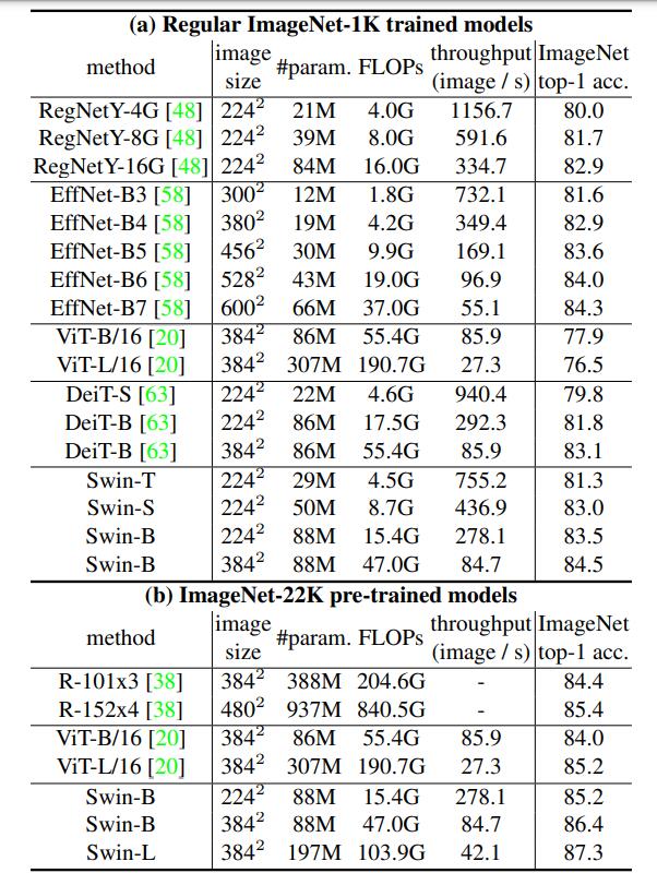
The first column is the comparison method, the second column is the size of the image (the larger the size, the greater the amount of floating-point operations), the third column is the amount of parameters, the fourth column is the amount of floating-point operations, and the fifth column is the model throughput. quantity. It can be seen that Swin-T surpasses most models in top1 accuracy. EffNet-B3 is indeed an excellent network. It is slightly better than Swin-T when the number of parameters and FLOPs are less than Swin-T. However, Based on the ImageNet1K dataset, Swin-B achieves the best results on these models. In addition, the top1 accuracy of Swin-L on ImageNet-22K has reached a height of 87.3%, which is not achieved by previous models. And other configurations of Swin Transformer have also achieved excellent results. The Swin Transformer with different configurations in the figure is explained as follows.

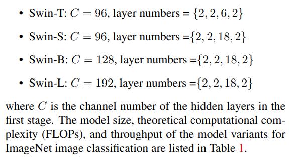
C is the value similar to the number of channels mentioned above, and layer numbers are the number of Swin Transformer Blocks. Both of these are the larger the value, the better the effect. Very similar to ResNet.

The figure below shows the performance of target detection and instance segmentation on the COCO dataset. All are comparisons of the same network under different backbone networks. It can be seen that under different APs, Swin Transformer has an improvement of about 5%, which is already an excellent level. No wonder it can become the best paer of ICCV2021.

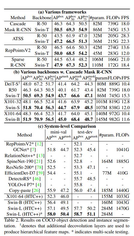
The figure below shows the performance on the semantic segmentation dataset ADE20K. Compared with DeiT-S, which is also a transformer, Swin Transformer-S has a 5% performance improvement. Compared with ResNeSt-200, Swin Transformer-L also has a 5% improvement. In addition, it can be seen that under the framework of UNet, all versions of Swin Transformer have excellent results, which fully demonstrates that Swin Transformer is a general backbone network in the CV field.

• ReferencesSwin
  Transformer

5.ViT( Vision Transformer-2020)

In the field of computer vision, most algorithms keep the overall structure of CNN unchanged, adding attention modules to CNN or using attention modules to replace some parts of CNN. Some researchers have suggested that it is not necessary to always rely on CNN. Therefore, the author proposes the ViT ^[1] algorithm, which can perform well in image classification tasks only using the Transformer structure.

Inspired by the successful application of Transformer in the NLP field, the ViT algorithm tries to apply the standard Transformer structure directly to images, and makes minimal modifications to the entire image classification process. Specifically, in the ViT algorithm, the entire image is split into small image blocks, and then the linear embedding sequence of these small image blocks is sent to the network as the input of the Transformer, and then image classification training is performed using supervised learning.

The algorithm was experimentally verified on medium-scale (such as ImageNet) and large-scale (such as ImageNet-21K, JFT-300M) data sets, and found that:

• Compared with the CNN structure, Transformer lacks certain translation invariance and local perception, so it is difficult to achieve the same effect when the amount of data is insufficient. Specifically, the Transformer trained with a medium-sized ImageNet will be several percentage points lower in accuracy than ResNet.
• The results change when there are a large number of training samples. After pre-training with a large-scale data set, it can be applied to other data sets by means of transfer learning, which can reach or exceed the current SOTA level.

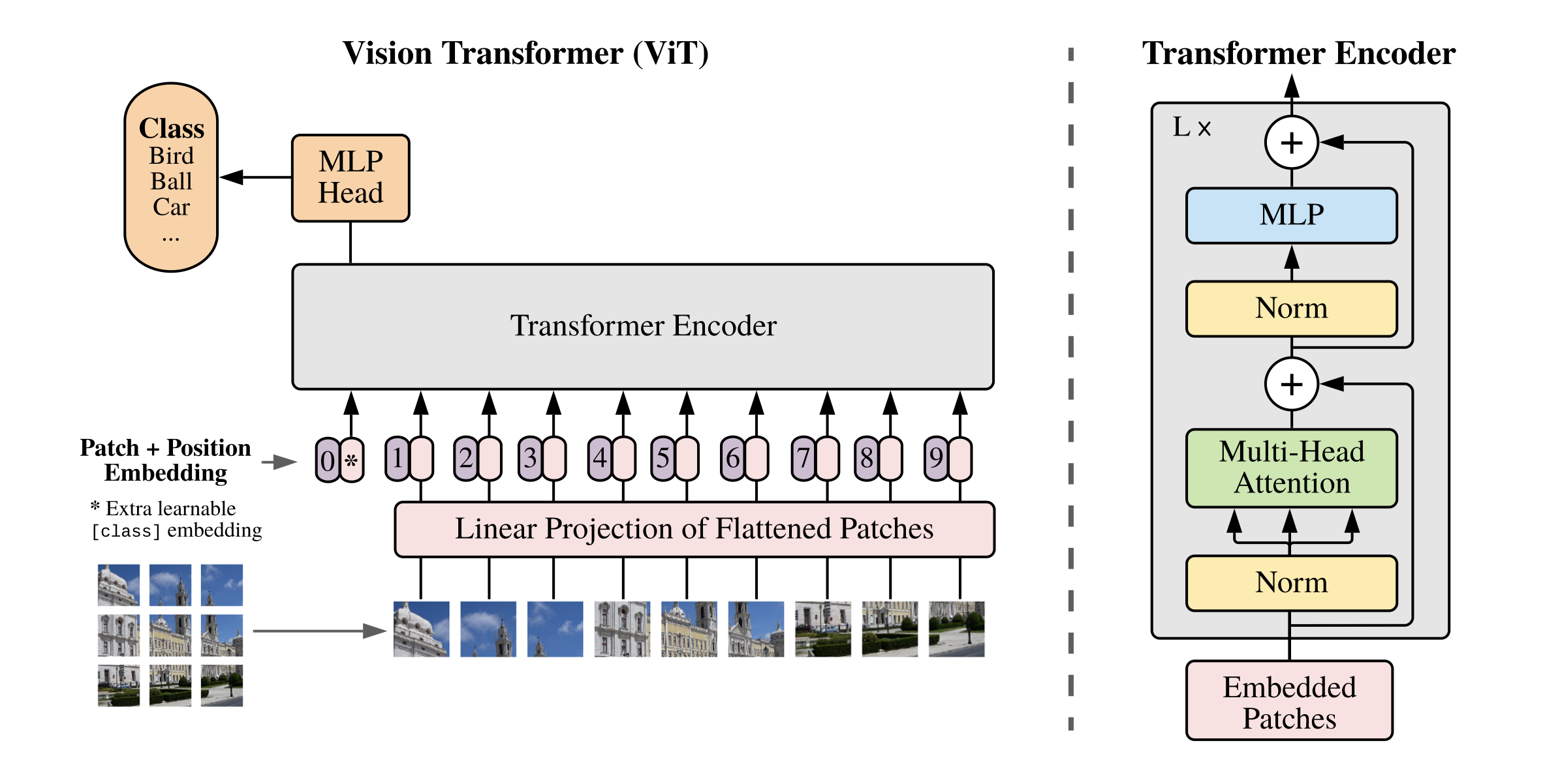
5.1 ViT model structure and realization

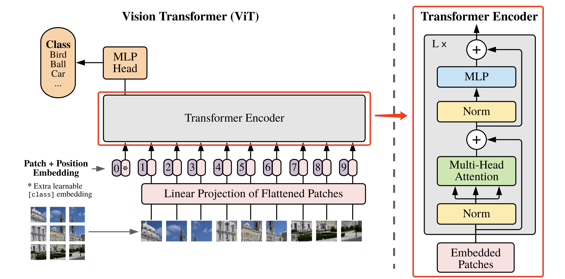
The overall structure of the ViT algorithm is shown in Figure 1.

5.1.1. ViT image block embedding

Considering that in the Transformer structure, the input is a two-dimensional matrix, the shape of the matrix can be expressed as $(N,D)$ , where$N$ is the length of the sequence, and$D$ is the dimension of each vector in the sequence. Therefore, in the ViT algorithm, it is first necessary to try to convert$H\times W\times The\; three-dimensional\; image\; of\; C$ is transformed into$(N,D)$ Two-dimensional input.

The specific implementation in ViT is: $H\times W\times The\; image\; of\; C$ becomes a$N\times (P^2\ast C)$ sequence. This sequence can be regarded as a series of flattened image blocks, that is, after the image is cut into small blocks, it is then flattened. The sequence contains a total of$N=HW/P^2$ image blocks, the dimension of each image block is$(P^2\ast C)$ . of which$P$ is the size of the image block,$C$ is the number of channels. After the above transformation, the NNcan be$N$ is regarded as the length of the sequence.

However, at this time the dimension of each image block is $(P^2\ast C)$ , and the vector dimension we actually need is$D$ , so we also need to Embedding the image block. The way of Embedding here is very simple, only need for each$(P^2\ast C)$ image blocks do a linear transformation to compress the dimension to$D$ is enough.

The above-mentioned specific way of dividing the image into blocks and embedding is shown in FIG. 2 .

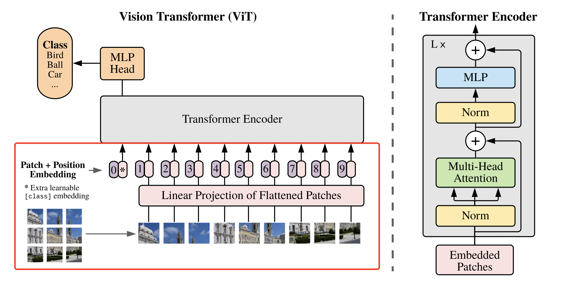
The specific code implementation is as follows. In this paper, each size is referred to as $The\; image\; block\; of\; P$ passes through the size ofPPThe convolution kernel of$P$$After\; the\; image\; block\; of\; P$ is flattened, it is followed by the operation of full connection operation.

#图像分块、Embedding
class PatchEmbed(nn.Layer):
    def __init__(self, img_size=224, patch_size=16, in_chans=3, embed_dim=768):
        super().__init__()
        # 原始大小为int，转为tuple，即：img_size原始输入224，变换后为[224,224]
        img_size = to_2tuple(img_size)
        patch_size = to_2tuple(patch_size)
        # 图像块的个数
        num_patches = (img_size[1] // patch_size[1]) * \
            (img_size[0] // patch_size[0])
        self.img_size = img_size
        self.patch_size = patch_size
        self.num_patches = num_patches
        # kernel_size=块大小，即每个块输出一个值，类似每个块展平后使用相同的全连接层进行处理
        # 输入维度为3，输出维度为块向量长度
        # 与原文中：分块、展平、全连接降维保持一致
        # 输出为[B, C, H, W]
        self.proj = nn.Conv2D(
            in_chans, embed_dim, kernel_size=patch_size, stride=patch_size)

    def forward(self, x):
        B, C, H, W = x.shape
        assert H == self.img_size[0] and W == self.img_size[1], \
            "Input image size ({H}*{W}) doesn't match model ({self.img_size[0]}*{self.img_size[1]})."
        # [B, C, H, W] -> [B, C, H*W] ->[B, H*W, C]
        x = self.proj(x).flatten(2).transpose((0, 2, 1))
        return x

5.1.2. ViT multi-head attention

Convert the image to $N\times (P^2\ast C)$ After the sequence, it can be input into the Transformer structure for feature extraction, asshown in Figure 3.

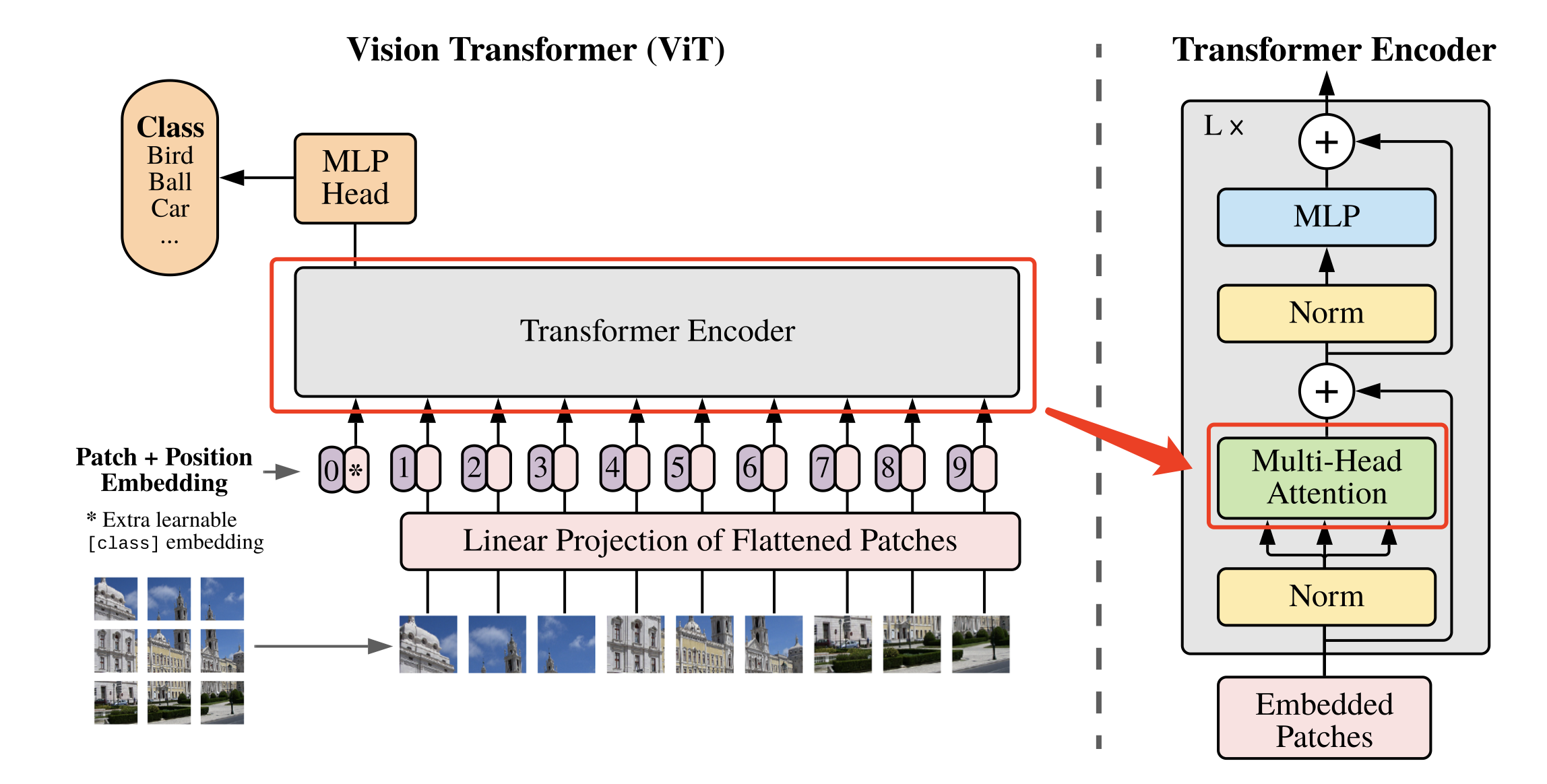
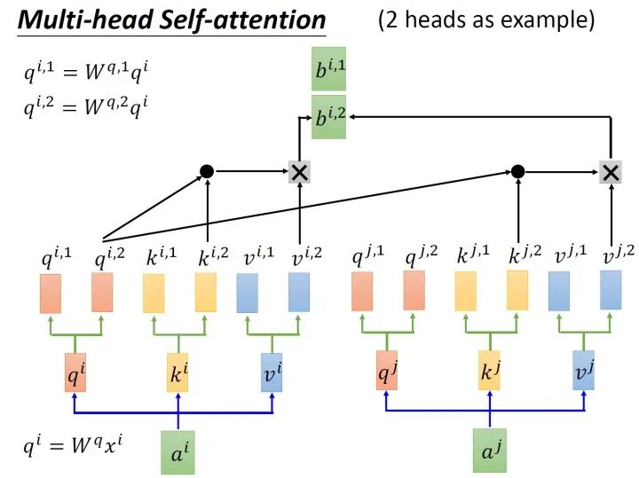
The most important structure in the Transformer structure is Multi-head Attention, that is, the multi-head attention structure. The Multi-head Attention structure with 2 heads is shown in Figure 4. Enter $a^i$ passes through the transfer matrix and splits to generate$q^{(i,1)}$、$q^{(i,2)}$、$k^{(i,1)}$、$k^{(i,2)}$、$v^{(i,1)}$、$v^{(i,2)}$ , after$q^{(i,1)}$ given$k^{(i,1)}$ do attention and get the weight vector$\alpha$ , will$\alpha$ given$v^{(i,1)}$ weighted sum to get the final$b^{(i,1)}(i=1,2,\dots ,N)$ , in the same way,$b^{(i,2)}(i=1,2,\dots ,N)$ . They are then concatenated and processed through a linear layer to get the final result.

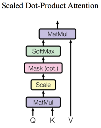
where, using $q^{(i,j)}$、$k^{(i,j)}$ given$v^{(i,j)}$计算$b^{(i,j)}(i=1,2,\dots ,N)$ method is Scaled Dot-Product Attention (Scaled Dot-Product Attention). The structure is shown in Figure. First use each$q^{(i,j)}$ go with$k^{(i,j)}$ do attention, the attention mentioned here is how close the two vectors are matched. The specific way is to calculate the weighted inner product of the vectors to get$a_{(i,j)}$. The weighted inner product calculation method here is as follows:

$$a_{(1,i)}=q^1\ast k^i/\sqrt{d}$$

Among them, $d$ is$q$ and$The\; dimension\; of\; k$ , since$q\ast The\; value\; of\; k$ will increase as the dimension increases, so divide by$\sqrt{d}$The value of is equivalent to the effect of normalization.

Next, the calculated $a_{(i,j)}$Take the softmax operation, and then combine it with $v^{(i,j)}$ multiplied together.

The specific code implementation is as follows.

#Multi-head Attention
class Attention(nn.Layer):
    def __init__(self,
                 dim,
                 num_heads=8,
                 qkv_bias=False,
                 qk_scale=None,
                 attn_drop=0.,
                 proj_drop=0.):
        super().__init__()
        self.num_heads = num_heads
        head_dim = dim // num_heads
        self.scale = qk_scale or head_dim**-0.5
        # 计算 q,k,v 的转移矩阵
        self.qkv = nn.Linear(dim, dim * 3, bias_attr=qkv_bias)
        self.attn_drop = nn.Dropout(attn_drop)
        # 最终的线性层
        self.proj = nn.Linear(dim, dim)
        self.proj_drop = nn.Dropout(proj_drop)

    def forward(self, x):
        N, C = x.shape[1:]
        # 线性变换
        qkv = self.qkv(x).reshape((-1, N, 3, self.num_heads, C //
                                   self.num_heads)).transpose((2, 0, 3, 1, 4))
        # 分割 query key value
        q, k, v = qkv[0], qkv[1], qkv[2]
        # Scaled Dot-Product Attention
        # Matmul + Scale
        attn = (q.matmul(k.transpose((0, 1, 3, 2)))) * self.scale
        # SoftMax
        attn = nn.functional.softmax(attn, axis=-1)
        attn = self.attn_drop(attn)
        # Matmul
        x = (attn.matmul(v)).transpose((0, 2, 1, 3)).reshape((-1, N, C))
        # 线性变换
        x = self.proj(x)
        x = self.proj_drop(x)
        return x

5.1.3. Multilayer Perceptron (MLP)

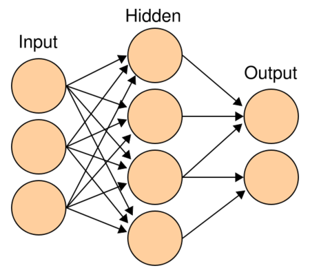
Another important structure in the Transformer structure is MLP, that is, multi-layer perceptron, as shown in Figure 6.

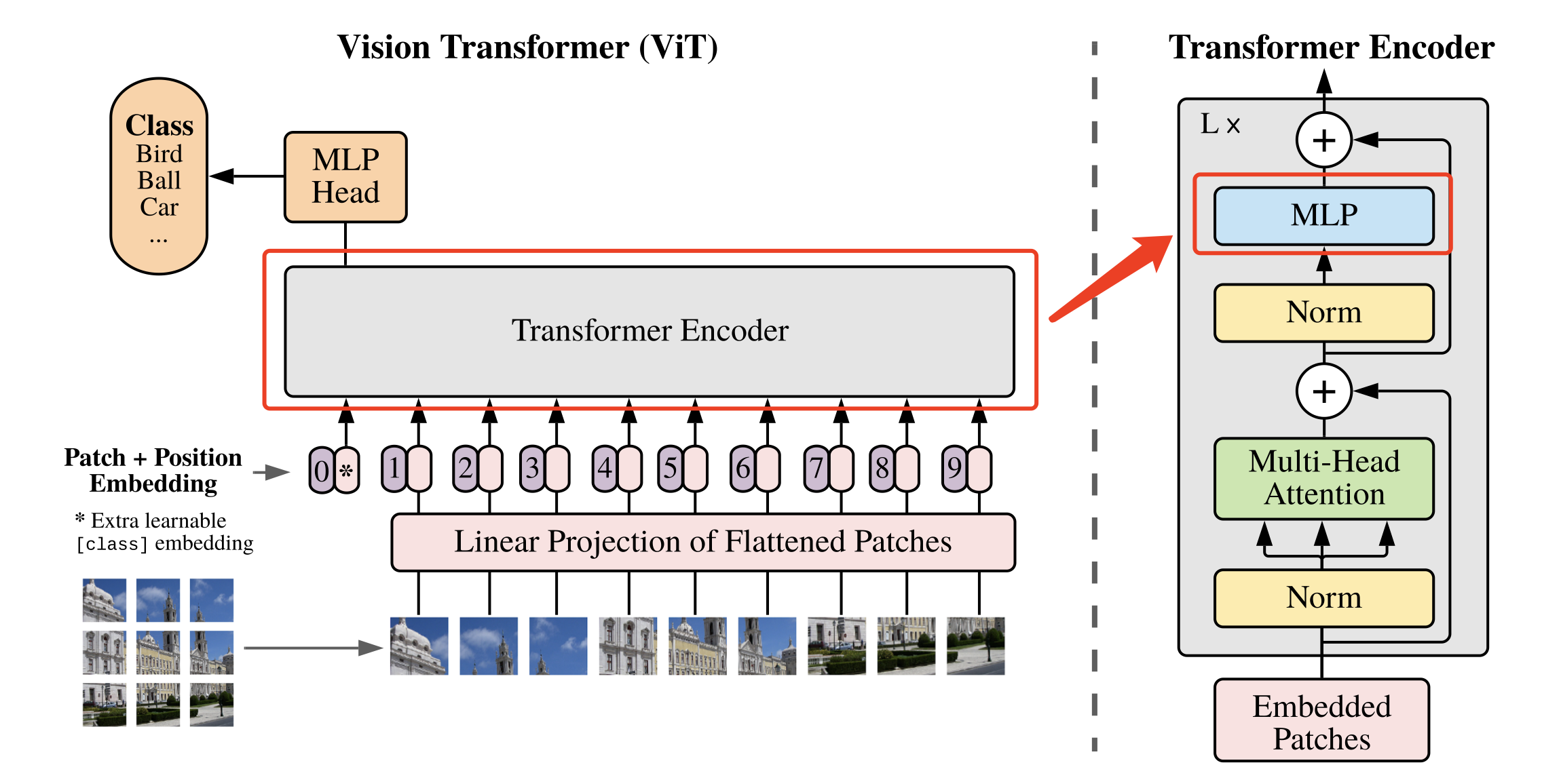
A multilayer perceptron consists of an input layer, an output layer, and at least one hidden layer. The neurons in each hidden layer in the network can receive the information transmitted by all the neurons in the adjacent preceding hidden layer, and output the information to all the neurons in the adjacent subsequent hidden layer after processing. In a multi-layer perceptron, neurons in adjacent layers are usually connected using a "full connection" method. Multi-layer perceptron can simulate complex nonlinear functions, and the complexity of the simulated functions depends on the number of hidden layers of the network and the number of neurons in each layer. The structure of the multi-layer perceptron is shown in Figure 7.

The specific code implementation is as follows.

class Mlp(nn.Layer):
    def __init__(self,
                 in_features,
                 hidden_features=None,
                 out_features=None,
                 act_layer=nn.GELU,
                 drop=0.):
        super().__init__()
        out_features = out_features or in_features
        hidden_features = hidden_features or in_features
        self.fc1 = nn.Linear(in_features, hidden_features)
        self.act = act_layer()
        self.fc2 = nn.Linear(hidden_features, out_features)
        self.drop = nn.Dropout(drop)

    def forward(self, x):
        # 输入层：线性变换
        x = self.fc1(x)
        # 应用激活函数
        x = self.act(x)
        # Dropout
        x = self.drop(x)
        # 输出层：线性变换
        x = self.fc2(x)
        # Dropout
        x = self.drop(x)
        return x

5.1.4. DropPath

In addition to the above important modules, DropPath (Stochastic Depth) is also used in the code implementation process to replace the traditional Dropout structure. DropPath can be understood as a special type of Dropout. Its role is to randomly drop a subset of layers during training, and use the full Graph normally during prediction.

The specific implementation is as follows:

def drop_path(x, drop_prob=0., training=False):
    if drop_prob == 0. or not training:
        return x
    keep_prob = paddle.to_tensor(1 - drop_prob)
    shape = (paddle.shape(x)[0], ) + (1, ) * (x.ndim - 1)
    random_tensor = keep_prob + paddle.rand(shape, dtype=x.dtype)
    random_tensor = paddle.floor(random_tensor)
    output = x.divide(keep_prob) * random_tensor
    return output

class DropPath(nn.Layer):
    def __init__(self, drop_prob=None):
        super(DropPath, self).__init__()
        self.drop_prob = drop_prob

    def forward(self, x):
        return drop_path(x, self.drop_prob, self.training)

5.1.5 Basic modules

Based on the Attention, MLP, and DropPath modules implemented above, a basic module of the Vision Transformer model can be combined, as shown in Figure 8.

The specific implementation of the basic module is as follows:

class Block(nn.Layer):
    def __init__(self,
                 dim,
                 num_heads,
                 mlp_ratio=4.,
                 qkv_bias=False,
                 qk_scale=None,
                 drop=0.,
                 attn_drop=0.,
                 drop_path=0.,
                 act_layer=nn.GELU,
                 norm_layer='nn.LayerNorm',
                 epsilon=1e-5):
        super().__init__()
        self.norm1 = eval(norm_layer)(dim, epsilon=epsilon)
        # Multi-head Self-attention
        self.attn = Attention(
            dim,
            num_heads=num_heads,
            qkv_bias=qkv_bias,
            qk_scale=qk_scale,
            attn_drop=attn_drop,
            proj_drop=drop)
        # DropPath
        self.drop_path = DropPath(drop_path) if drop_path > 0. else Identity()
        self.norm2 = eval(norm_layer)(dim, epsilon=epsilon)
        mlp_hidden_dim = int(dim * mlp_ratio)
        self.mlp = Mlp(in_features=dim,
                       hidden_features=mlp_hidden_dim,
                       act_layer=act_layer,
                       drop=drop)

    def forward(self, x):
        # Multi-head Self-attention， Add， LayerNorm
        x = x + self.drop_path(self.attn(self.norm1(x)))
        # Feed Forward， Add， LayerNorm
        x = x + self.drop_path(self.mlp(self.norm2(x)))
        return x

5.1.6. Define the ViT network

After the basic modules are constructed, a complete ViT network can be constructed. Before building a complete network structure, we need to introduce several modules:

• Class Token

Suppose we divide the original image into $3\times 3$ There are 9 small image blocks in total, but the final input sequence length is 10, which means that we artificially add a vector for input here, and we usually call this artificially added vector Class Token. So what is the function of this Class Token?

We can imagine that without this vector, that is, $N=9$ vectors are input into the Transformer structure for encoding, and we will finally get 9 encoding vectors, but for the image classification task, which output vector should we choose for subsequent classification? Therefore, the ViT algorithm proposes a learnable embedding vector Class Token, which is input into the Transformer structure together with 9 vectors, and 10 coded vectors are output, and then the Class Token is used for classification prediction.

In fact, it can also be understood here: ViT actually only uses the Encoder in the Transformer, but does not use the Decoder, and the role of the Class Token is to find the categories corresponding to the other 9 input vectors.

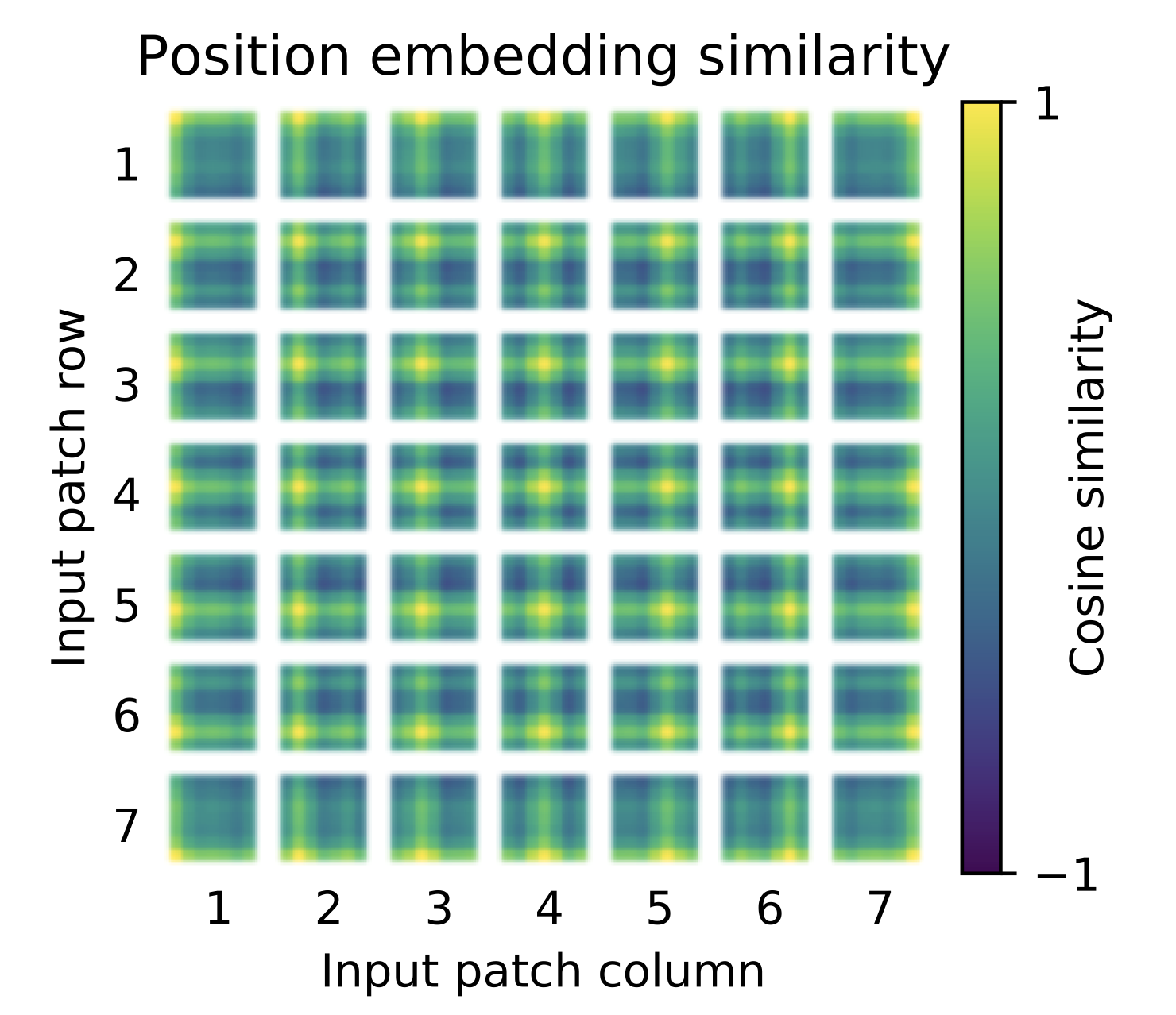
• Positional Encoding

According to the positional encoding convention in the Transformer structure, this work also uses positional encoding. The difference is that the position encoding in ViT does not use $sincos$ encoding, but directly set to learnable Positional Encoding. Visualize the trained Positional Encoding, asshown in Figure 9. We can see that closer locations tend to have more similar location encodings. Furthermore, a row-column structure emerges, with patches in the same row/column having similar positional encodings.

• MLP Head

After the output is obtained, the MLP Head is used in ViT to classify the output. The MLP Head here is composed of LayerNorm and two fully connected layers, and the GELU activation function is used.

The specific code is as follows.

First build the basic module part, including: parameter initialization configuration, an independent network layer that does not perform any operations.

#参数初始化配置
trunc_normal_ = nn.initializer.TruncatedNormal(std=.02)
zeros_ = nn.initializer.Constant(value=0.)
ones_ = nn.initializer.Constant(value=1.)

#将输入 x 由 int 类型转为 tuple 类型
def to_2tuple(x):
    return tuple([x] * 2)

#定义一个什么操作都不进行的网络层
class Identity(nn.Layer):
    def __init__(self):
        super(Identity, self).__init__()

    def forward(self, input):
        return input

The full code is shown below.

class VisionTransformer(nn.Layer):
    def __init__(self,
                 img_size=224,
                 patch_size=16,
                 in_chans=3,
                 class_dim=1000,
                 embed_dim=768,
                 depth=12,
                 num_heads=12,
                 mlp_ratio=4,
                 qkv_bias=False,
                 qk_scale=None,
                 drop_rate=0.,
                 attn_drop_rate=0.,
                 drop_path_rate=0.,
                 norm_layer='nn.LayerNorm',
                 epsilon=1e-5,
                 **args):
        super().__init__()
        self.class_dim = class_dim

        self.num_features = self.embed_dim = embed_dim
        # 图片分块和降维，块大小为patch_size，最终块向量维度为768
        self.patch_embed = PatchEmbed(
            img_size=img_size,
            patch_size=patch_size,
            in_chans=in_chans,
            embed_dim=embed_dim)
        # 分块数量
        num_patches = self.patch_embed.num_patches
        # 可学习的位置编码
        self.pos_embed = self.create_parameter(
            shape=(1, num_patches + 1, embed_dim), default_initializer=zeros_)
        self.add_parameter("pos_embed", self.pos_embed)
        # 人为追加class token，并使用该向量进行分类预测
        self.cls_token = self.create_parameter(
            shape=(1, 1, embed_dim), default_initializer=zeros_)
        self.add_parameter("cls_token", self.cls_token)
        self.pos_drop = nn.Dropout(p=drop_rate)

        dpr = np.linspace(0, drop_path_rate, depth)
        # transformer
        self.blocks = nn.LayerList([
            Block(
                dim=embed_dim,
                num_heads=num_heads,
                mlp_ratio=mlp_ratio,
                qkv_bias=qkv_bias,
                qk_scale=qk_scale,
                drop=drop_rate,
                attn_drop=attn_drop_rate,
                drop_path=dpr[i],
                norm_layer=norm_layer,
                epsilon=epsilon) for i in range(depth)
        ])

        self.norm = eval(norm_layer)(embed_dim, epsilon=epsilon)

        # Classifier head
        self.head = nn.Linear(embed_dim,
                              class_dim) if class_dim > 0 else Identity()

        trunc_normal_(self.pos_embed)
        trunc_normal_(self.cls_token)
        self.apply(self._init_weights)
    # 参数初始化
    def _init_weights(self, m):
        if isinstance(m, nn.Linear):
            trunc_normal_(m.weight)
            if isinstance(m, nn.Linear) and m.bias is not None:
                zeros_(m.bias)
        elif isinstance(m, nn.LayerNorm):
            zeros_(m.bias)
            ones_(m.weight)
    
    def forward_features(self, x):
        B = paddle.shape(x)[0]
        # 将图片分块，并调整每个块向量的维度
        x = self.patch_embed(x)
        # 将class token与前面的分块进行拼接
        cls_tokens = self.cls_token.expand((B, -1, -1))
        x = paddle.concat((cls_tokens, x), axis=1)
        # 将编码向量中加入位置编码
        x = x + self.pos_embed
        x = self.pos_drop(x)
        # 堆叠 transformer 结构
        for blk in self.blocks:
            x = blk(x)
        # LayerNorm
        x = self.norm(x)
        # 提取分类 tokens 的输出
        return x[:, 0]

    def forward(self, x):
        # 获取图像特征
        x = self.forward_features(x)
        # 图像分类
        x = self.head(x)
        return x

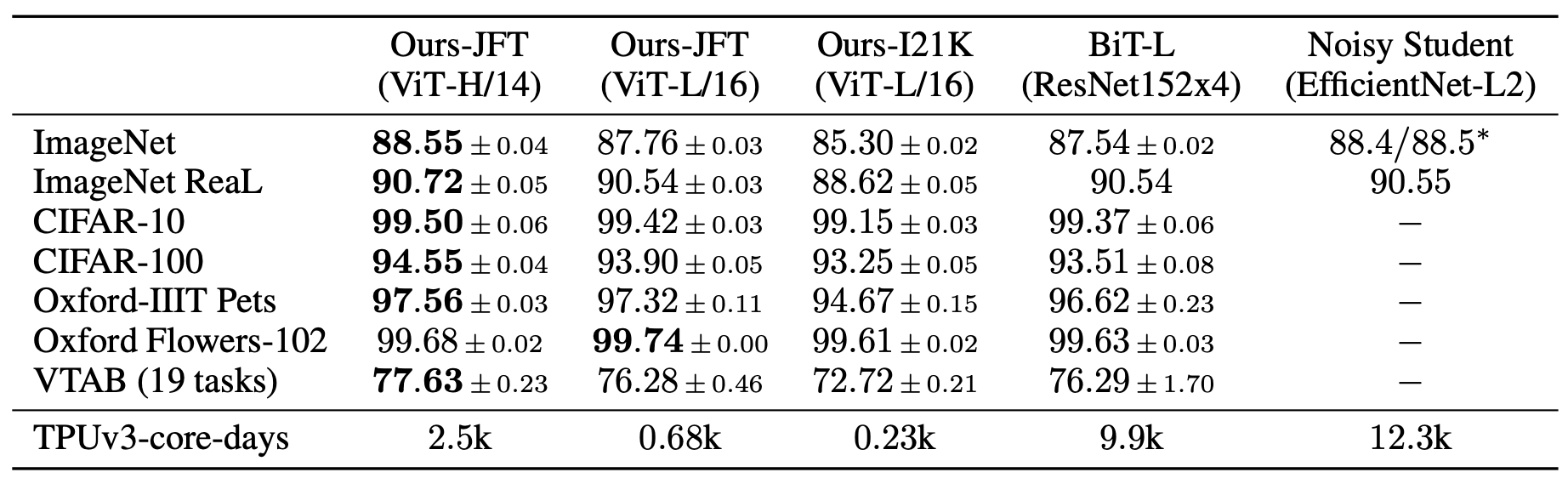
5.2 ViT model indicators

The ViT model performs transfer learning on common datasets, and the final indicators are shown in Figure 10. It can be seen that on ImageNet, the highest index reached by ViT is 88.55%; on ImageNet ReaL, the highest index reached by ViT is 90.72%; on CIFAR100, the highest index reached by ViT is 94.55%; on VTAB (19 tasks) On the above, the highest index achieved by ViT is 88.55%.

5.3 Features of ViT model

• As one of the most classic Transformer algorithms in the CV field, unlike the traditional CNN algorithm, ViT tries to apply the standard Transformer structure directly to images, and makes minimal modifications to the entire image classification process.
• In order to meet the requirements of the Transformer input structure, the entire image is split into small image blocks, and then the linear embedding sequence of these small image blocks is input to the network. At the same time, Class Token is used for classification prediction.

• references

[1] An Image is Worth 16x16 Words:Transformers for Image Recognition at Scale