【Paper Reading】GRAF_ Generative Radiance Fields for 3D-Aware Image Synthesis

Paper: http://arxiv.org/abs/2007.02442
Code: https://github.com/autonomousvision/graf

Summary

2D Generative Adversarial Networks can achieve high-resolution image synthesis, but cannot be well applied to 3D image synthesis. To solve this problem, several methods combining intermediate voxel-based representation with differentiable rendering have emerged, but these methods suffer from several problems: 1) the synthesized images are of low resolution; 2) in terms of separating camera and scene attributes It has a shortpart.
This paper presents a generative model of radiation fields that has been shown to be successful in novel view synthesis of single scenes. In contrast to voxel-based representations, the radiation field is not restricted to a coarse discretization of 3D space, but instead allows the decomposition of camera and scene properties while gracefully degrading in the presence of reconstruction ambiguities. By introducing a multi-scale patch-based discriminator, the model in this paper is only trained on unprocessed 2D images, and high-resolution image synthesis can also be achieved.

1 Introduction

Although convolutional GANs can achieve high-resolution image synthesis from unordered image collections, state-of-the-art models still struggle to correctly decompose basic generative factors including 3D shape and viewpoint. Humans, by contrast, have the ability to reason about the three-dimensional structure of the world and to imagine objects from new perspectives.
Since 3D reasoning is fundamental for robotics, virtual reality, or data augmentation applications, the task of image synthesis that considers 3D perception arises with the goal of generating realistic images by explicitly controlling the pose of the camera. In contrast to 2D GANs, methods for 3D-aware image synthesis learn a 3D scene representation that is explicitly mapped onto the image using a differentiable rendering technique, thus providing control over scene content and perspective.
However, 3D supervised or placed images are often difficult to obtain in practice, so only 2D supervision is considered to solve this task. Existing methods use discrete 3D representations, such as voxel-grid representing complete 3D objects or intermediate 3D features to achieve this goal, as shown in Figure 1 below:

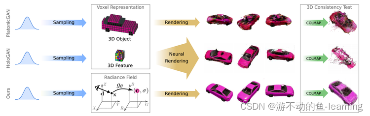
                                        "图 1  Motivation"        

While modeling 3D objects in color space can take advantage of differential rendering, the limitation of cubic memory growth of voxel-based representations makes it possible to synthesize only low-resolution images and leads to visible artifacts. intermediate 3D features are more compact and have better image resolution. But this requires learning a 3D-to-2D mapping for decoding abstract features into RGB values, which leads to inconsistencies between views at high resolutions.

1.1 Contribution of this paper

1. GRAF designs a conditional variant of the NeRF representation, showing how to learn a rich generative model from a set of unposed 2D images. In addition to viewpoint operations, it also allows modifying the shape and appearance of generated objects.
2. Introducing a patch-based discriminator that samples images at multiple scales is the key to effectively learning high-resolution generative NeRF.

2 Related Work

2.1 Image Synthesis

GANs significantly advance photorealistic image synthesis to a remarkable level. But 2D images are obtained as projections of the 3D world. Although there are some methods that show that disentangled factors capture some 3D properties to a certain extent, it is still very difficult to model image manifolds with 2D convolutional networks, especially multi-view. Consistent and seek representations that reliably separate viewpoint changes from object appearance and identity. Therefore, this paper takes the approach of generating 3D representations and explicitly modeling the image formation process.

2.2 3D-aware image synthesis

2.3 Implicit representation

Implicit representation of 3D geometry has been popularized in learning-based 3D reconstruction, and its main advantage over voxel- or grid-based methods is that it does not discretize space and is not limited by topology. NeRF represents the scene as a neural radiance field, which allows multi-view-consistent novel view synthesis of more complex real-world scenes from posed 2D images. Inspired by NeRF, this paper designs a conditional variant of the NeRF representation, GRAF, and shows how to learn a rich generative model from a set of unposed 2D images as input.

3 Method

3.1 Neural Radiance Fields（NeRF）

For details, refer to the blog: https://blog.csdn.net/KeepLearning1/article/details/129923446

3.2 Generative Radiance Fields

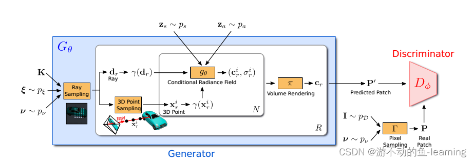
                                            "图 2 GRAF的整体框架"

The overall framework of GRAF is shown in Figure 2. Similar to GAN, GRAF is divided into Generator $G_{}$和Discriminator $D_{}$two parts. The generator part will be the camera matrix $K$ , camera pose$\xi$ , 2D sampling template$v$ and shape/appearance encoding$z_s\in R^m/z_a\in R^n$ as input, and predict an image patch$P^{\prime }$ , where each Ray consists of$K,x,v$ Three input decisions, the conditional radiance field is the only part of the generator that can be learned. The discriminator predicts the synthetic patch$P^{\prime }$ and real image sampling to get real patch$P$ makes a judgment. In the training phase, GRAF uses sparse$K\times The\; fixed\; patch\; of\; K$ pixels is efficiently optimized, and the test phase predicts the color value of each pixel of the target image. (If the color value of each pixel value is also predicted during training, the cost is too high)

3.2.1 Generator

From the attitude distribution $p_{}$Medium sampling camera pose (pose) $X=[R|t]$ , in the experiments in this paper, the uniform distribution of the hemisphere is used as the camera position, and the camera faces the origin of the coordinate system. Uniformly varies the distance from the camera to the origin, depending on the dataset. Also choose K so that the principal point is at the center of the image.
$n=(u,s)$ determines$K\times K$个patch$P(u,s)$ center position$u=(u，v)\in R^2$ and scale$s\in R^{+}$ .
This enables the use of convolutional discriminators that are independent of image resolution. From the image domainω ωRandomly draw the patch centeru ∼ U ( ω ) u \sim U(ω)$from\; a\; uniform\; distribution\; on\; \omega$$u\sim U\left(\omega \right)$ , and from the uniform distribution$s\sim$Randomly draw the scaless$of\; the\; patch\; in\; U$$([$$1$$,$$S$$])$$s$ , where$S=min(W,H)/K$ , where W and H represent the width and height of the target image. Furthermore, ensure that the entire patch is within the image domain ω. shape and appearance variables$z_s$sum $z_a$from the shape and appearance distributions $z_s\sim p_s$和$z_a\sim p_a$. In the experiments in this paper $p_{s}and{p}_a$are standard Gaussian distributions.

Ray Sampling

$P(u,s)$ is determined by a sequence of 2D image coordinates:

the corresponding 3D rays are given by$P(u,s)$ , camera matrix$K$ , camera pose$\xi$ is uniquely determined according to$n=(u,s)$ , sampling$R=k^2$ rays, inference stage sampling$R=WH$ Rays.
3D point Sampling
for the numerical integration of the radiation field, along each ray$r$ sampling N points$\left\{x_r^i\right\}$ . Like NeRF, the hierarchical sampling method is adopted (for details, refer to:https://blog.csdn.net/KeepLearning1/article/details/129923446)
Conditional Radiance Fields
The radiation field is represented by a deep fully connected neural network (MLP), Its parameter$\theta$ will be the three-dimensional position$x\in R^3$ and the viewing direction$d\in S^{The\; positional\; code\; of\; 2}$ maps to the RGB color value$c$ and bulk density$\sigma$ :


Compared with the original NeRF formula,$g_{}$Conditional on two additional latent codes: 1) The shape code $z_s\in R^{M_s}$;2) The appearance code za ∈ RM a z_a \in R^{M_a} that determines the appearance of the object$z_a\in R^{M_a}$. Therefore, it is said that $g_{}$is the conditional radiance fields
$g_{}$The structure of is shown in Figure 4, starting from the position code $\gamma (x)$和shape code$z_s$Calculate the shape encoding $h$ , density head$p_{}$Convert this encoding to the bulk density $\sigma$ . To predict a color c at a 3D position x, encode the position of h with d$\gamma \left(d\right)$ and appearance code$z_a$concatenated, and pass the resulting vector to the color head $c_{}$. Independent of viewpoint d and appearance code $z_a$calculation $\sigma$ to encourage multi-view consistency while separating shape from appearance. This encourages the network to use the latent code$z_s$sum $z_a$Model shape and appearance separately and allow them to be manipulated independently during inference.

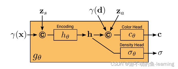
The above process is expressed as follows:

All maps ( $h_{}、c_{}和p_{}$) are implemented using fully connected networks with ReLU activations.
Volume Rendering
Given the color and volume density of all points along the ray r $(c_r^i,p_r^i)$ , use the rendering operation in the following formula to obtain the color$c_r\in R^3$ . .combine all$The\; result\; of\; R$ rays, denoting the predicted patch as$P^{’}$ , as shown in Figure 2.

3.2.2 Discriminator

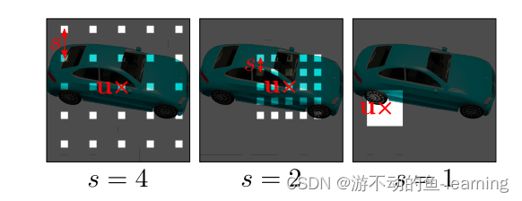
Discriminator $D_{}$is implemented as a convolutional neural network (see table2 for details), which predicts the patch $P^{\prime }$ and from the data distribution$p_D$Real image drawn in IIThe patch PPextracted in$I$$P$ for comparison. In order to get from the real image$I$ extract$K\times K$ patches, first from the same distribution p ν p_νused to draw the patches of the generator above$p_{}$中运动$n=(u,s)$ . Then, by using bilinear interpolation at the 2D image coordinates$P(u,s)$ query$I$ come to the real patch$P$ is sampled. In the following, use$C(I,\nu )$ to represent this bilinear sampling operation. The discriminator is similar to PatchGAN, and our method allows continuous displacement u and scaling s while PatchGAN uses s = 1. It is more important to note that our method does not downsample the real image I according to s, but instead queries I at sparse locations to preserve high-frequency details, see Figure 3. Through experiments, the authors found that a single discriminator with shared weights is sufficient to

use for all patches, even if these patches are sampled at random locations with different scales. Because the scale determines the receptive field of the patch. Therefore, to facilitate training, start with patches with larger receptive fields to capture the global context. Then, patches with smaller receptive fields are progressively sampled to improve local details.

3.2.3 Training and Inference

$I$ means from the data distribution$p_D$the image of $p_{}$Represents a distribution over random patches (see Section 3.2.1). Train the model using an unsaturated GAN objective with R1 regularization:

where $f(t)=-log(1+exp(-t))$，$\lambda$ controls the strength of the regularizer. Spectral normalization and instance normalization are used in the discriminator, and our method is trained using RMSprop with a batch size of 8 and learning rates of 0.0005 and 0.0001 for the generator and discriminator, respectively. At inference time, randomly sample$z_s、z_{a}and\xi$ , and predict the color values ​​of all pixels in the image.

4 experiments

Datasets
Two synthetic datasets:

• Photoshapes, 150K chair
• CarlaDriving, 10K images of 18 car models with randomly sampled colors and realistic texture and reflection properties

Three real-world datasets:

• Image synthesis at resolutions up to 1282 and 5122 pixels using the Faces dataset containing celebA and celebA-HQ, respectively
• Cats dataset
• Caltech-UCSD Birds-200-2011 dataset

Baseline
compares our method with two state-of-the-art models for 3D-aware image synthesis implemented by the original authors:

• PLATONICGAN Generates voxel meshes of 3D objects, volume rendering using differentiable projection to image plane
• HoloGAN generates an abstract voxelized feature representation and uses a combination of 3D and 2D convolutions to learn a 3D-to-2D mapping
• A modified version of HoloGAN (HoloGAN w/o 3D Conv) is further considered, where the capacity of the learned map is reduced by removing the 3D convolutional layers
• For reference, the results of this paper are also compared with the state-of-the-art 2D GAN model with ResNet architecture

Evaluation Metrics

• Frechet Inception Distance (FID), quantifying image fidelity
• Kernel Inception Distance (KID)
• Minimum Matching distance (MMD) to measure the chamfer distance (CD) between 100 reconstructed shapes and their closest shape in ground truth for quantitative comparison and to show qualitative results of the reconstruction.

In the following, several key issues related to the algorithm of this paper are studied.

4.1 How does generating a radiation field compare to voxel-based methods?

Use a resolution of $64^{2-}$ pixel images to compare our model with the baseline, as shown in Figure 5, all methods are able to distinguish between object identity and camera viewpoint. However, PLATONICGAN has difficulty representing thin structures, and both PLATONICGAN and HoloGAN lead to visible artifacts compared to GRAF. This is also illustrated by the larger FID scores in Table 1.


On Faces and Cats, HoloGAN achieves similar FID scores to GRAF, as these two datasets exhibit only small variations in camera azimuth, while the other datasets cover larger viewpoint variations. This shows that due to HoloGAN's low-dimensional 3D feature representation and learnable projections, it is more difficult to accurately capture the appearance of objects from different angles. In contrast, GRAF's continuous representation does not require learning projections and renders high-fidelity images from arbitrary views.

4.2 Can generative models for 3D perception scale to high-resolution output?

Due to the use of voxel-based representations, PLATONICGAN becomes very memory-intensive when encountering high-resolution images. Therefore, only GRAF is compared with HoloGAN and HoloGAN without 3D Conv. Training with $128^2$ resolution, inference is sampled at a higher resolution, at$128^2-512^{between\; 2}$ .

The results in Table 2 show that the GRAF approach significantly improves upon naive bilinear upsampling, which suggests that the representations learned by GRAF generalize well to higher resolutions. GRAF achieves the smallest FID value when trained at full resolution. HoloGAN without 3D Conv achieves comparable results to GRAF on the Faces dataset with small viewpoint changes.

4.3 Should learning to predict be avoided?

As shown in Figure 6, HoloGAN is unable to separate viewpoint from appearance at high resolution, alter different stylistic aspects such as facial expressions, or even completely ignore pose input. The authors identify learnable projections as the root cause of this behavior. In particular, the authors found that removing the 3D convolutional layers enabled HoloGAN to more closely obey the input pose, see Figure 6 (middle). To better study multi-view consistency, multiple images of the same instance at random viewpoints are generated for HoloGAN w/o 3D Conv and GRAF methods, and dense 3D reconstruction is performed using COLMAP. Since reconstruction depends on the consistency between views, the reconstruction accuracy can represent the multi-view consistency of the generated images. From Table 3 and Figure 7, it is evident that the multi-view stereo effect is significantly better when using images in GRAF as input. In contrast, HoloGAN without 3D Conv can build fewer correspondences, which uses learned 2D layers for upsampling. For HoloGAN with 3D convolutions, the performance drops further, as shown in the figure below. Therefore, the authors conjecture that learning predictions should generally be avoided.

4.4 Can generating a radiation field separate shape from appearance?

In addition to disentangling camera and scene properties, GRAF also learns to disentangle shape and appearance, which can be controlled by zs and za during inference. For Cars and Chairs, the appearance code controls the object's color, while for Faces it encodes the color of the skin and hair.

4.5 How important is the multi-scale patch discriminator?

A multi-scale patch discriminator is compared with (Patch) with a discriminator (Full) that receives the entire image as input. Since this is very memory intensive, only consider a resolution of $64^2$ , and for$h_{}and{c}_{}(dim/2)$ uses half the hidden dimension. Table 4 shows that our multi-scale patch discriminator achieves similar performance to the full image discriminator on Cars, and performs even better on CelebA. A possible explanation for this phenomenon is that random patch sampling, as a data augmentation strategy, helps stabilize GAN training. In contrast, when only local patches (s = 1) are used, the multi-scale patch discriminator cannot learn the correct shape, resulting in high FID values ​​in Table 4. The authors therefore conclude that sampling patches at random scales is critical for robust performance.

5 Conclusion

This paper introduces a generative radiative field (GRAF) for high-resolution 3D perceptual image synthesis. Experiments show that GRAF is able to generate high-resolution images with better multi-view consistency compared to voxel-based methods. However, this is limited to simple scenes with a single object . Incorporating inductive biases, such as depth maps or symmetries, will allow our model to scale to more challenging real-world scenarios in the future.