1. Integrated algorithm
Integrated algorithm : Ensemble learning (ensemble learning) itself is not a separate machine learning algorithm, but completes learning tasks by building and combining multiple machine learners , so it often has more significant generalization performance than a single learner.
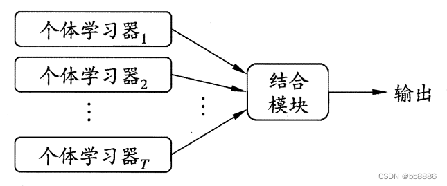
The general structure of integrated learning: first generate a set of "individual learners", and then combine them with a certain strategy. Individual learners are usually generated from training data by an existing learning algorithm.
According to the generation method of individual learners, the current ensemble learning can be mainly divided into two categories: ①There is a strong dependency between individual learners, and the serialization method that must be generated serially, the representative is Boosting (boosting); ②Individual learners There is no strong dependency between them, and the parallelization method can be generated at the same time. The representatives are Bagging (bagging) and random forest .
Two, Boosting
Introduction : Boosting is a family of algorithms that can upgrade a weak learner to a strong learner. The most famous representative of the Boosting family of algorithms is AdaBoost (adaptive boost).
AdaBoost : The adaptiveness of AdaBoost is that the weights of samples misclassified by the previous basic classifier will increase, while the weights of correctly classified samples will decrease, and are used again to train the next basic classifier . At the same time, in each round of iterations, a new weak classifier is added, and the final strong classifier is not determined until a predetermined small enough error rate is reached or a pre-specified maximum number of iterations is reached . In layman's terms, it is the process of accumulating several weak classifiers with weights to obtain a strong classifier.
Working mechanism : first train a base learner from the initial training set, and then adjust the distribution of training samples according to the performance of the base learner, so that the training samples that the previous base learner made mistakes will receive more attention in the follow-up, and then based on the adjusted The sample distribution of the next base learner is used to train the next base learner; this is repeated until the number of base learners reaches the value T specified in advance, and finally the T base learners are weighted and combined.
The Boosting algorithm learns a specific data distribution through the "re-weighting" method . For basic learning algorithms that cannot accept weighted samples, it can be dealt with by "re-sampling" . Boosting mainly focuses on reducing bias, so Boosting can build strong integration based on learners with relatively weak generalization performance .
3. Bagging and Random Forest
There is no strong dependency between individual learners, that is, individual learners should be as independent as possible and have as large a difference as possible.
How to achieve a large difference? The training sample is sampled to generate several different subsets, and then a base learner is trained from each data subset. Considering that the generated subsets may be completely different, that is to say, each base learner only uses a small part of the training data, which is not even enough for effective learning, which obviously cannot ensure a better base learner. Consider using overlapping sampling subsets .
1. Bagging : Bagging uses a sampling method with replacement to generate training data. Through multiple rounds of random sampling of the initial training set with replacement, multiple training sets are generated in parallel, and correspondingly multiple base learners can be trained (there is no strong dependency between the base learners ), and then these base learners Machines are combined to build a strong learner. Its essence is to introduce sample disturbance, and achieve the effect of reducing variance by increasing sample randomness .
Bagging typically uses simple voting for classification tasks and simple averaging for regression tasks when combining predicted outputs .
2. Random Forest RF : It is an extended variant of Bagging. On the basis of building Bagging ensemble with decision tree as the base learner, RF further introduces random attribute selection in the training process of decision tree.
(1) Sample selection is random. For the original training set of m samples, we randomly collect a sample into the sampling set each time, and then put the sample back, that is to say, the sample may still be collected in the next sampling, so that m times are collected, Finally, a sampling set of m samples can be obtained. Since it is a random sampling, each sampling set is different from the original training set, and also different from other sampling sets, so that multiple different weak learners are obtained.
(2) Node selection is random. When selecting a partition attribute in a traditional decision tree, an optimal attribute is selected from the attribute set of the current node (according to criteria such as information gain, gain rate, etc.), while in RF, for each node of the base decision tree, start with Randomly select a subset containing K attributes from the attribute set of the node, and then select an optimal attribute from this subset for division. The parameter k here controls the degree of randomness introduced, and k=log(d) is recommended.
4. GBDT
Introduction: GBDT, full name Gradient Boosting Decision Tree, gradient boosting tree. It mainly consists of two parts: Gradient Boosting and Decision Tree .
1. Decision Tree: CART regression tree.
What are CARTs? The full name of CART is Classification and Regression Tree, a well-known decision tree learning algorithm, both classification and regression tasks are available.
Why not use a CART classification tree? Whether it is a regression problem or a classification problem, GBDT needs to accumulate the results of multiple weak classifiers, and each iteration needs to fit the gradient value, which is a continuous value, so a regression tree is used, that is to say, DT refers to Regression alone. Decision Tree.
What is the criterion for the best division point of the regression tree? Classification tree: entropy or Gini coefficient. Regression Trees: Squared Error.
2. Gradient Boosting: Fitting negative gradient
Gradient Boosting : The gradient direction of a function is the direction in which the function rises fastest, and conversely, the negative gradient direction is the direction in which the function descends the fastest. The gradient promotion here is actually a kind of idea of gradient descent .
Gradient boosting algorithm : Use the approximation method of the steepest descent, that is, use the value of the negative gradient of the loss function in the current model as an approximation of the residual of the boosting tree algorithm in the regression problem to fit a regression tree.
A training method of boosting- residual-based training . Keep the existing model, and we will continue to solve the part that this model cannot solve. This is the training method based on the residual. Although each model is relatively weak, at least we can ensure that each of them is somewhat useful, which is better than random guessing.
Residual-based training can solve problems similar to the following: ( residuals - problems that cannot be solved yet )
(1) Given a prediction problem, Zhang San trained a model - "Model1" on this data, but the effect is not very good, the error is relatively large, how to receive this model but can not make any changes?
(2) After taking over a project, one of the colleagues gave some plans, but they were not perfect, and we couldn’t ask him to change them, and we couldn’t stop using his plans. What should we do?
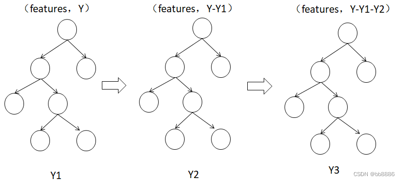
The principle of boosting tree : use the next weak classifier to fit the current residual (true value - current predicted value), and then add the results of all weak classifiers to be equal to the predicted value. In GBDT, the expression form of the weak classifier here is CART tree. As shown in the figure Y = Y1 + Y2 + Y3.
For Boosting Tree, why is it summed instead of averaged in the final decision?
For the regression problem, if we learn a lot of decision trees according to the residual method, it is actually different from Bagging in the prediction stage, because in Bagging, each tree is trained independently and does not affect each other, so the final decision needs to be voting decisions. But boosting is different. Boosting training is serial , one after another, and the training of each tree depends on the previous residuals . Based on these characteristics, we should require sums instead of averages for Boosting.
3、GBDT
3.1 Principle
GBDT, Gradient Boosting Decision Tree, is an iterative decision tree algorithm. The algorithm consists of multiple decision trees, and the conclusions of all trees are accumulated to make the final answer . It was considered to be an algorithm with strong generalization ability (generalization) together with SVM when it was proposed. In recent years, it has attracted everyone's attention because of the machine learning model used for search ranking.
3.2 GBDT regression task [Example 1]
Someone is 30 years old this year, but the computer or model GBDT does not know how old he is, so what should GBDT do?
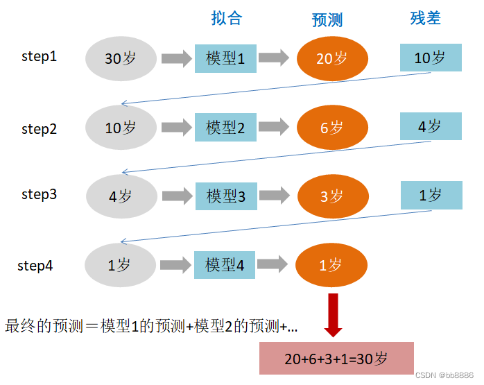
Step 1: In the first tree, use a random age (20 years old) to fit, and find that the error is 10 years old (10=30-20); Step 2: In the
second tree, use 6 years old To fit the remaining loss, it is found that the gap is still 4 years old;
the third step: in the third tree, fit the remaining gap with 3 years old, and find that the gap is only 1 year old; the
fourth step: in the fourth In the class tree, use 1 year old to fit the remaining residuals, perfect.
In the end, the sum of the conclusions of the four trees is the real age of 30 years (in actual engineering, gbdt calculates the negative gradient and uses the negative gradient to approximate the residual ).
Why can gbdt approximate residuals with negative gradients?
The loss function under the regression task is the mean square error loss function: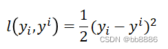
Its negative gradient calculation formula is:![]()
Therefore, when the mean square loss function is selected as the loss function, the value of each fitting is (true value - value predicted by the current model), that is, the residual error.
3.3 GBDT regression task [Example 2]
Assume that there are only 4 people in the training set: A, B, C, and D, and their ages are 14, 16, 24, and 26 respectively. Among them, A and B are high school students and high school students respectively; C and D are fresh graduates and working students respectively. For two-year employees, the problem is predicting age.
If a traditional regression decision tree is used for training, the results shown in the following figure are obtained:
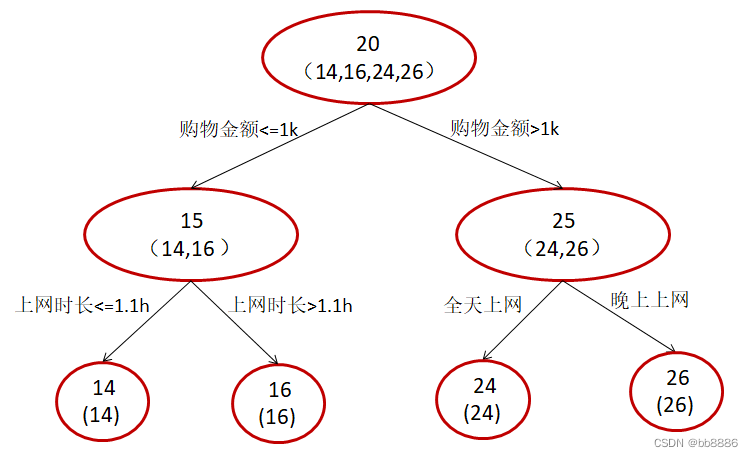
We use GBDT to predict age, limit up to two leaf nodes, and limit learning to only two trees.

The first branch of the tree is the same as that in Figure 1. Since A and B are relatively similar in age, and C and D are relatively similar in age, they are divided into left and right groups, and the average age of each group is used as the predicted value . Further, the residuals of A, B, C, and D are -1, 1, -1, and 1, respectively.
A: A 14-year-old high school student who does not shop much, often asks seniors questions, predicted age A = 15 – 1 = 14
B: 16-year-old high school student, does little shopping, often asked questions by students, predicted age B = 15 + 1 = 16
C: 24-year-old fresh graduate, shopping a lot, often asks seniors questions, predicted age C = 25 – 1 = 24 D
: 26-year-old employee who has worked for two years, does a lot of shopping, often asked questions by seniors, predicted age D = 25 + 1 = 26
GBDT needs to accumulate the scores of multiple trees to obtain the final prediction score, and each iteration, on the basis of the existing tree, add a tree to fit the residual between the prediction result of the previous tree and the real value.
3.4 GBDT classification task
There is no difference between the classification algorithm and the regression algorithm of GBDT, but because the sample output is not a continuous value, but a discrete category, we cannot directly fit the error of the category output from the output category.
Solution:
With the exponential loss function, GBDT degenerates into the Adaboost algorithm at this time.
Use a method similar to the log-likelihood loss function of logistic regression (divided into binary and multivariate classification).
3.5 The difference between GBDT and LR
(1) Both are supervised learning, Logisitic Regression (LR) is a classification model, and GBDT can be used for both classification and regression.
(2) Loss function: The loss of LR is cross entropy, GBDT uses regression fitting (converting the classification problem into a regression problem through softmax), and uses the current loss to fit the residual between the actual value and the predicted value of the previous round of model .
(3) From the perspective of regularity: LR adopts l1 and l2 regularization; GBDT adopts the number of weak classifiers, that is, iteration round T, and the size of T affects the complexity of the algorithm.
(4) Feature combination: LR is a linear model, which has good interpretability and is easy to parallelize. It is not a problem to process hundreds of millions of training data, but the learning ability is limited and requires a lot of feature engineering; GBDT can handle linear and nonlinear Data has natural advantages for feature combination.