The purpose of this article is to explain Flash Attention in detail, why explain Flash Attention? Because FlashAttention is an algorithm for reordering attention computation, it can speed up attention computation and reduce memory footprint without any approximation. Therefore, as the current LLM model acceleration, it is a very good solution. This article introduces the classic V1 version, and the latest V2 has other optimizations that we will not introduce here for the time being. Because the V1 version of FlashAttention is claimed to be 5-10 times faster, so let's study how it is implemented.
introduce
The title of the paper is:
“FlashAttention: Fast and Memory-Efficient Exact Attention with IO-Awareness”
Memory efficiency Compared to normal attention (sequence length is quadratic, O(N²)), FlashAttention is subquadratic/linear N (O(N)). And it is not an approximation of attention mechanisms (e.g. sparse or low-rank matrix approximation methods) - its output is the same as "traditional" attention mechanisms. Compared with ordinary attention, FlashAttention's attention is "perceived".
It leverages knowledge of the memory hierarchy of the underlying hardware (e.g. GPUs, but other AI accelerators should work too, I'm using GPUs here as an example). Some [approximate] methods reduce computational requirements to linear or near-linear in sequence length, but many of them focus on reducing FLOPs while ignoring the overhead of memory access (IO).
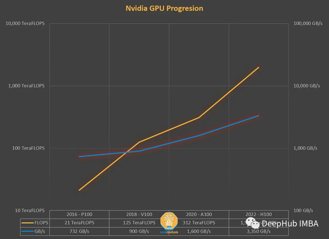
After years of development, the FLOPS of GPUs has been growing faster than the memory throughput (TB/s). Memory bottlenecks should be taken seriously. FLOPS and memory throughput need to be closely combined. Due to the gap in hardware, we need to balance the work at the software level.
Depending on the ratio between computation and memory access, operations can be classified into the following two types:
- Computational Constraints: Matrix Multiplication
- Memory constraints: element operations (activation, dropout, masking), merge operations (softmax, layer norm, sum, etc.)
On the current AI accelerator (GPU), it is limited by the memory size. Because it "majorly consists of element-wise operations", or more precisely, the arithmetic density of attention is not very high.
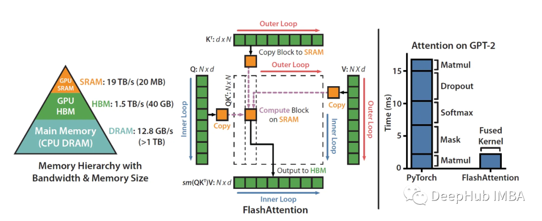
Let's look at this picture:
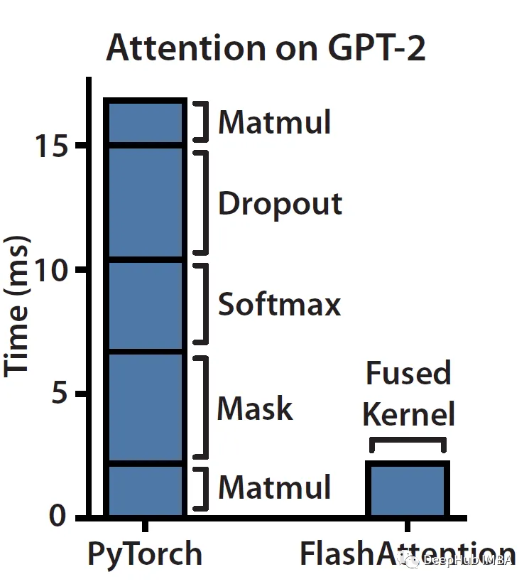
As you can see, masking, softmax, and dropout are time-consuming operations, not matrix multiplication (even though most of the FLOPS are in matmul). Memory is not a single artifact, it is hierarchical in nature, and the general rule is: the faster the memory, the more expensive it is, the smaller the capacity.
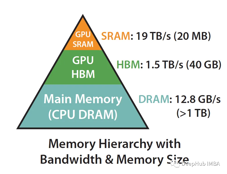
What we said above that FlashAttention's attention is "aware" boils down to utilizing SRAM much faster than HBM (High Bandwidth Memory) to ensure less communication between the two.
Take A100 as an example:
The A100 GPU has 40-80GB of high-bandwidth memory (HBM), with a bandwidth of 1.5-2.0 TB/s, while each of the 108 stream processors has 192KB of SRAM, and the bandwidth is estimated to be around 19TB/s.
It can be seen that the size is much smaller, but the speed is increased by 10 times, so how to efficiently use SRAM is the key to speeding up. Let us look at the calculation behind the implementation of standard attention:
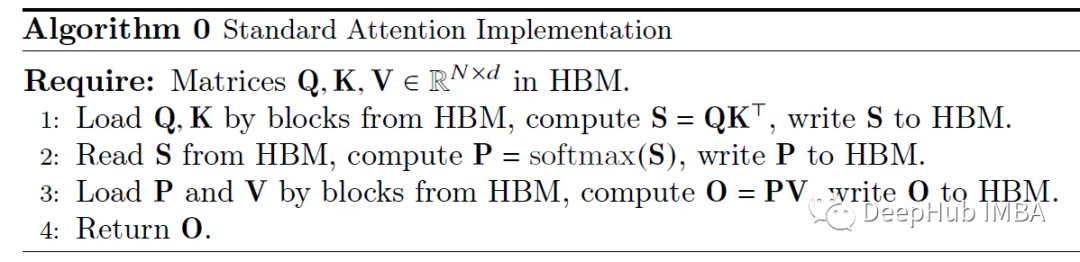
How the standard implementation shows little respect for how HW operates. It basically treats HBM load/store operations as 0 cost (it's not "io aware").
We first consider how to make this implementation more efficient (in terms of time and memory). The easiest way is to remove redundant HBM reads/writes.
How about writing S back to HBM just to (re)load it to compute softmax, then we can keep it in SRAM, perform all intermediate steps, and then write the final result back to HBM.
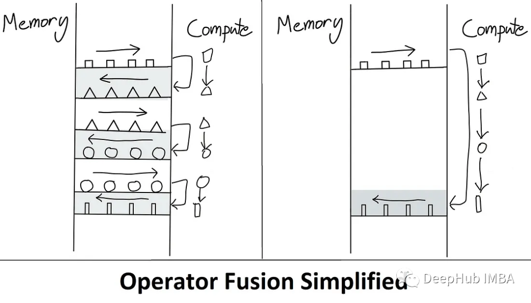
A kernel is basically a fancy way of saying "GPU operations" (refer to our previous post on Getting Started with CUDA, which is simply a function). Fusion allows multiple operations to be fused together. So only load once from HBM, execute the fused op, and write the result back. Doing so reduces communication overhead.
There is also a technical term here is "materialization" (materialization / materialization). It refers to the fact that, in the standard attention implementation above, the full NxN matrix (S, P) has been allocated. Below we will see how to directly reduce the memory complexity from O(N²) to O(N).
Flash attention basically boils down to two main points:
Tiling (used during forward and backward pass) - basically tiling the NxN softmax/scores matrix into chunks.
Recomputation (only used in the backward pass)
The algorithm is as follows:

We mentioned a lot of nouns above, which you may not understand yet. It doesn't matter, let's start to explain the algorithm line by line.
Flash Attention Algorithm
The main obstacle to the Tiling method is softmax. Because softmax needs to couple all the score columns together.
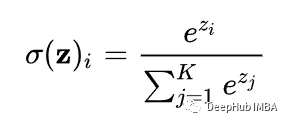
See the denominator? That's the problem.
Computing how much attention a particular i-th token in the input sequence has to other tokens in the sequence requires all of these scores (denoted here by z_j) to be readily available in SRAM.
But the capacity of SRAM is limited. N (sequence length) can be 1000 or even 100000 tokens. So N² explodes very quickly. So the paper uses a trick: divide the calculation of softmax into smaller blocks, and still get exactly the same result in the end.

We can just take the previous B scores (x_1 to x_B) and compute softmax for them. Then through iterations, "converge" to the correct result. Combining these per-block softmax numbers in a clever way, such that the final result is actually correct. Methods as below:

Basically, in order to compute the softmax of the scores belonging to the first 2 blocks (of size B), one has to keep track of 2 statistics for each block: m(x) (max score) and l(x) (sum of exp scores) . They can then be seamlessly blended together using normalization coefficients.
Here are mainly some basic algebraic operations. By expanding the f(x) and l(x) terms and multiplying them with e^x, some terms will cancel each other out, so I won’t write them here. This logic continues recursively until the last (N/B) block, which results in an N-dimensionally correct softmax output!
For the sake of detailing this algorithm, assume a batch of size 1 (i.e. a single sequence) and a single attention head, which will later be extended (by simple parallelization across GPUs - more on that later). We ignore dropout and masking for now, as they will be added later.

We start calculating:
Initialization: The capacity of HBM is measured in GB (e.g. RTX 3090 has 24 GB of VRAM/HBM, A100 has 40-80 GB, etc.), so allocating Q, K and V is not a problem.
step 1
Calculate row/column block size. Why ceil(M / 4 d) ? Because the query, key, and value vectors are d-dimensional, we also need to combine them into the output d-dimensional vector. So this size basically allows us to maximize the capacity of SRAM with qkv and 0 vectors.
For example, suppose M = 1000, d = 5. Then the block size is (1000/4*5)=50. So load 50 blocks of q, k, v, o vectors at a time, which can reduce the number of read/writes between HBM/SRAM.
For B_r, I'm also not quite sure why they are using d to perform the minimum operation? If anyone knows, please comment and advise!
Step 2:

Initialize the output matrix O with all zeros. It will act as an accumulator, l similarly its purpose is to hold the cumulative denominator of the softmax - the sum of exp scores). M (holding the row-by-row max score) is initialized to -inf because we'll be doing the Max operator on it, so whatever the Max of the first block is - it's definitely greater than -inf.
Step 3:

The block size in step 1 divides Q, K, and V into blocks.
Step 4:

Divide O, l, m into blocks (same block size as Q).
Step 5:
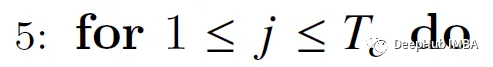
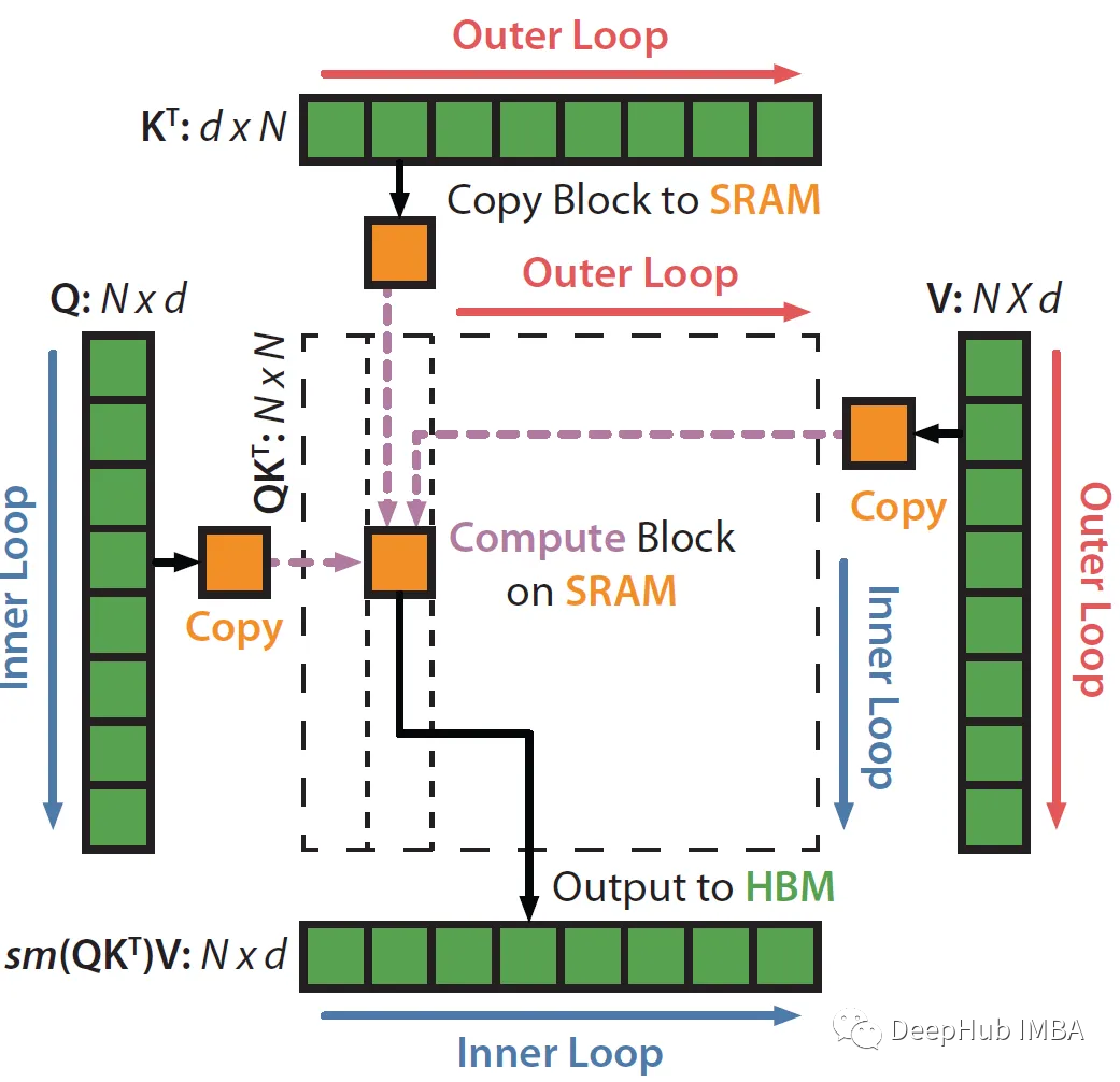
Start looping across columns, i.e. across key/value vectors (outer loop in the diagram above).
Step 6:

Load K_j and V_j blocks from HBM to SRAM. At this point in time we still have 50% of SRAM free (dedicated to Q and O). So SRAM is like this:
Step 7:
Start the inner loop across rows, i.e. across the query vector.
Step 8:

Load Q_i (B_r xd) and O_i (B_r xd) blocks and l_i (B_r) and m_i (B_r) into SRAM.
Here you need to ensure that l_i and m_i can be loaded into SRAM (including all intermediate variables), this may be CUDA knowledge, I am not sure how to calculate, so if you have relevant information, please leave a message
Step 9:

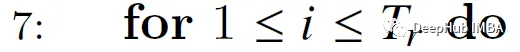
Compute the dot product between Q_i (B_r xd) and the K_j transpose (dx B_c) to get the score (B_r x B_c). does not "materialize" the entire nxns(score) matrix.
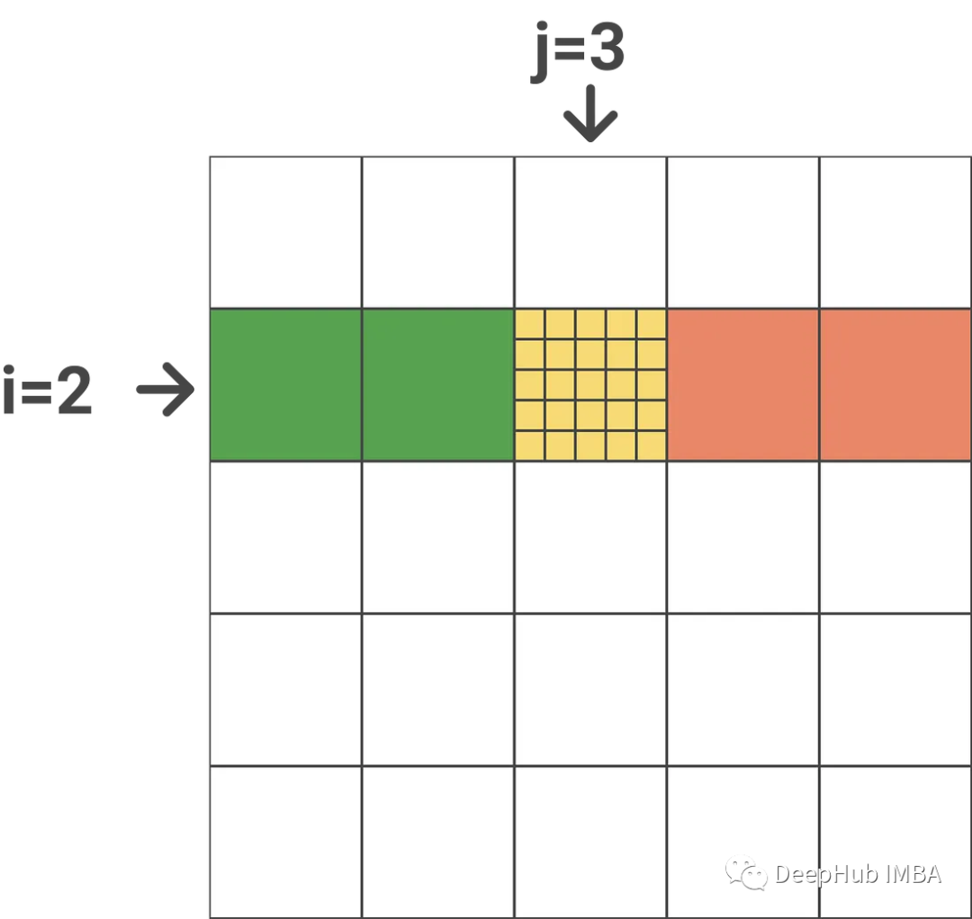
Assuming the outer loop index is j (j=3), the inner loop index is i (i=2), N is 25, and the block size is 5, the following is the result just calculated (assuming 1-based indexing):

That is, the attention scores for tokens 6-10 of tokens 11-15 in the input sequence. An important point here is that these are exact scores, they never change.
Step 10:

Calculate m_i_j, l*i_j and P~*i_j using the scores calculated in the previous step. M ~_i_j is computed row by row, finding the largest element of each row above.
Then P~_i_j is obtained by applying element-wise operations:
Normalize - take the row max and subtract it from the row score, then EXP
l~_i_j is the row-by-row sum of matrix P.
Step 11:

Calculate m_new_i and l_new_i. Also very simple to reuse the diagram above:
M_i contains the row-by-row maxima of all previous blocks (j=1 & j=2, denoted in green). M_i_j contains the row-by-row maximum value (indicated in yellow) for the current block. In order to get m_new_i we only need to take a maximum value between m_i_j and m_i, and l_new_i is similar.
Step 12 (most important):

This is the hardest part of the algorithm.
It allows us to do row-wise scalar multiplication in matrix form. If you have a column of scalars s(N) and a matrix a(NxN) if you do diag(s)*a you are basically doing element-wise multiplication of row a with those scalars.
Formula 1 (pasted here again for convenience):
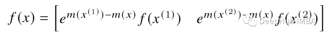
What the first item of step 12 does (underlined in green) is: it updates the current softmax estimate for the block preceding the current block in the same row block. if j=1 (This is the first block of this line.
The first term is multiplied by diag(l_i) to cancel out the same constant that was divided by in the previous iteration (this constant is hidden in O_i).
The second term of the expression (yellow underline) does not need to be eliminated, because we can see that we directly multiply the P~_i_j matrix with the V vector block (V_j).
The e^x term is used to modify the matrix P~_i_j & O_i by eliminating m from the previous iteration and updating it with the latest estimate (m_new_i) containing the row-by-row maximum so far.
Here's my step-by-step analysis (actually only takes 5 minutes, hope it helps!)

The point is that these outer e-terms and the e-terms in the P/O matrix are eliminated, so you always get the latest m_new_1 estimate!
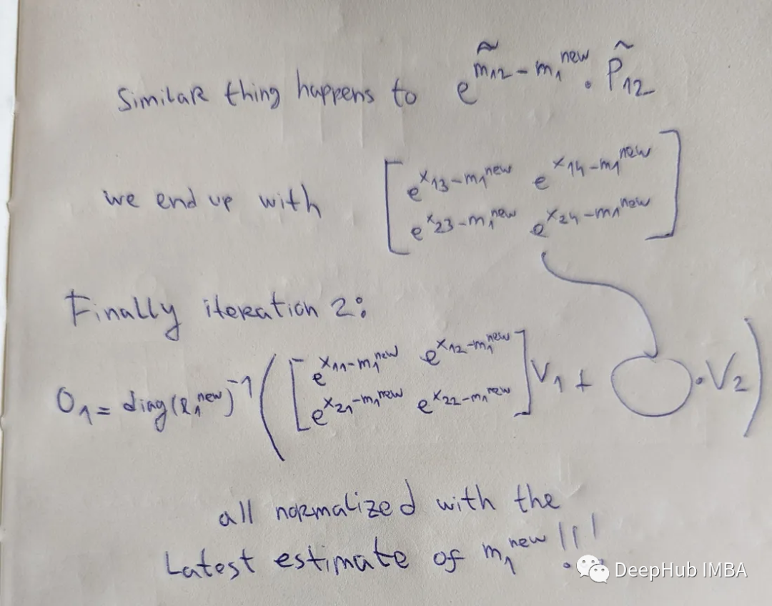
The third iteration was similar and got the correct final result!
Recall: this is only a current estimate of the final O_i. Only after we iterate through all the red blocks in the image above can we finally get the exact result.
step 13

Write the latest accumulated to statistics (l_i & m_i) back to HBM. Note that their dimensionality is B_r.
Steps 13, 14, 15, 1
End of nested for loops, O(Nxd) will contain the final result: a vector of attention weights for each input token!
simple summary
The algorithm can be easily extended to "block-sparse FlashAttention", which is a sparse attention algorithm that is 2-4 times faster than FlashAttention, and scales to sequence lengths of 64k! By using a mask matrix in block form, it is possible to skip Some load/store in the nested for loop above, so that we can save the sparse coefficient proportionally, such as the following figure

Now let's briefly discuss complexity.
Complexity Analysis
Space: Q, K, V, O (Nxd), l and m (N) are allocated in HBM. It is equal to 4 N d + 2*N. Removing the constant, and knowing that d is also a constant and usually much smaller than N (e.g. d={32,64,128}, N={1024,...,100k}), gives O(N) space, which helps Scales up to 64k sequence length (plus some other "tricks" like ALiBi).
Time: Time complexity analysis will not be done strictly here, but we will use a good metric: the number of HBM accesses.
The explanation of the paper is as follows:

How did they get this number? Let's analyze the nested for loops:
Our block size is M/4d. This means the vector is split into N/(M/4d) blocks. Taking it to the power of 2 (since you're traversing blocks of rows/columns) gives you O(N²d²/M²)
We can't fetch the whole block at once, and doing a big-oh analysis might lead us to think that this isn't much better than standard attention, but for typical numbers this results in a 9x reduction in the number of accesses (according to the paper screenshot above).
Our pseudo-algorithm focuses on a single-head attention, assuming a batch size of 1. Now we start to expand
multi-headed attention
It's actually not that hard to scale to batch_size > 1 and num_heads > 1.
Algorithms are basically processed by a single thread block (CUDA programming term). This thread block is executed on a single streaming multiprocessor (SM) (for example, there are 108 such processors on the A100). To parallelize computations, only batch_size * num_heads thread blocks need to be run in parallel on different SMs. The closer this number is to the number of SMs available on the system, the higher the utilization (ideally multiple, since each SM can run multiple thread blocks).
backpropagation
For the occupation of GPU memory, another big head is backpropagation. By storing the output O (Nxd) and softmax normalized statistics (N), we can directly reverse the Q, K and V (Nxd) blocks in SRAM. Computing the attention matrices S(NxN) and P(NxN) ! thus keeping the memory at O(N). This is more professional, we can understand the following, so please refer to the original paper for detailed content.
Code
Finally, let's look at some of the problems that can arise when using flash attention. Because it involves the operation of video memory, we can only go deep into CUDA, but CUDA is more complicated.
This is the strength of projects like OpenAI's Triton (see their implementation of FlashAttention). Triton is basically a DSL (Domain Specific Language), a level of abstraction between CUDA and other Domain Specific Languages such as TVM. It is possible to write super-optimized Python code (once compiled) without having to deal with CUDA directly. This way Python code can be deployed on any accelerator (this is the Triton task).
Another piece of good news is that Triton has recently been integrated with PyTorch 2.0.
Also for some use cases, like for sequence lengths over 1K, some approximate attention methods (like Linformer) start to become faster. But the block-sparse implementation of flash attention outperforms all other methods.
Summarize
Have you ever wondered why a student of Stanford University released the algorithm for this kind of bottom-level optimization instead of an engineer of NVIDIA?
I think there are 2 possible explanations:
1. FlashAttention is easier/only implementable on latest gpu (original codebase doesn't support V100).
2. Usually "outsiders" are those who look at problems with the eyes of beginners, can see the root of the problem and solve the problem from the basic principles
Finally, we still have to make a summary
FlashAttention can save 15% in BERT-large training, increase the GPT training speed by 2/3, and without modifying the code, this is a very important advancement, and it proposes a new one for LLM research direction.
Paper address:
https://avoid.overfit.cn/post/9d812b7a909e49e6ad4fb115cc25cdc1
Author: Aleksa Gordic