Improved module of YOLOv8 algorithm

Improved module of YOLOv8

YOLOv8 is the latest version of the YOLO (You Only Look Once) object detection and image segmentation model developed by Ultralytics. It is mainly based on YOLOv5 for algorithm improvement. The specific improvements are as follows:

YOLOv5 Core

1.Backbone：

CSPDarkNet structure, the main structural idea is reflected in the C3 module, where the main idea of ​​gradient shunting is located;

2.PAN-FPN：

Dual-stream FPN must be delicious and fast, but quantization still requires graph optimization to achieve optimal performance, such as scale optimization before and after cat, etc. In addition to upsampling and CBS convolution modules, the most important ones are C3 module;

3.List itemHead：

Coupled: Head+Anchor-base, there is no doubt that YOLOv3, YOLOv4, YOLOv5, and YOLOv7 are all Anchor-Base;

4.Loss：

BEC Loss is used for classification and CIoU Loss is used for regression.

YOLOv8 core content introduction

First look at the network structure diagram of YOLOv8

You can see the improvement as follows:

1. Backbone：

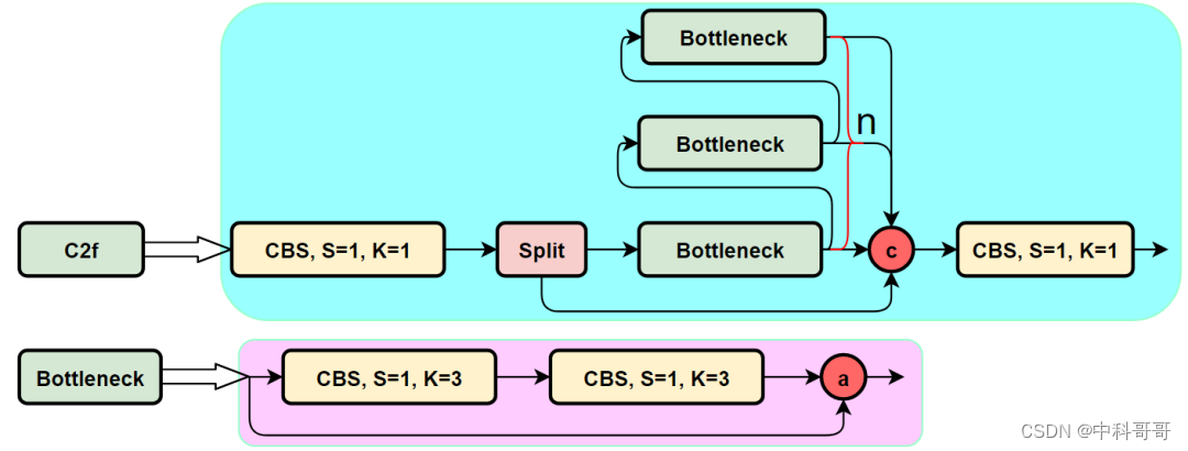
The idea of ​​CSP is still used, but the C3 module in YOLOv5 is replaced by the C2f module to achieve further lightweight, and YOLOv8 still uses the SPPF module used in YOLOv5 and other architectures;

2. PAN-FPN：

There is no doubt that YOLOv8 still uses the idea of ​​​​PAN, but by comparing the structure diagrams of YOLOv5 and YOLOv8, we can see that YOLOv8 deletes the convolution structure in the PAN-FPN upsampling stage in YOLOv5, and also replaces the C3 module with C2f module;

3. Decoupled-Head：

Did you smell something different? Yes, YOLOv8 went to Decoupled-Head;

4. Anchor-Free：

YOLOv8 abandoned the previous Anchor-Base and used the idea of ​​Anchor-Free;

5. Loss function:

YOLOv8 uses VFL Loss as classification loss and DFL Loss+CIOU Loss as classification loss;

6. Sample matching:

YOLOv8 abandoned the previous IOU matching or unilateral ratio allocation, but used the Task-Aligned Assigner matching method.

C2f module

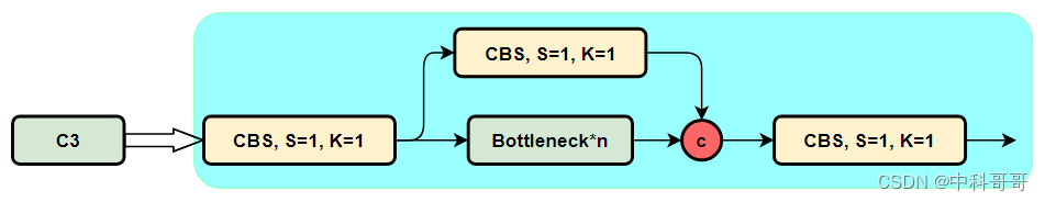
First look at the structure diagram of the C3 module, and then compare the specific differences with C2f. For the C3 module, it mainly uses CSPNet to extract the idea of ​​shunting, and at the same time combines the idea of ​​​​the residual structure to design the so-called C3 Block. The CSP main branch gradient module here is the BottleNeck module, which is the so-called residual module. The number of stacks at the same time is controlled by the parameter n, that is to say, the value of n varies for models of different scales.

In fact, the main branch of the gradient flow here can be any module you have learned before. For example, in YOLOv6, the re-reference module RepVGGBlock is used to replace the BottleNeck Block as the main gradient flow branch. PP-YOLOE uses RepResNet-Block to replace the BottleNeck Block as the main gradient flow branch. YOLOv7 uses ELAN Block to replace BottleNeck Block as the main gradient flow branch.

The Pytorch implementation of the C3 module is as follows:

class BottleneckC2f(nn.Module):
    # Standard bottleneck
    def __init__(self, c1, c2, shortcut=True, g=1, k=(3, 3), e=0.5):  # ch_in, ch_out, shortcut, kernels, groups, expand
        super().__init__()
        c_ = int(c2 * e)  # hidden channels
        self.cv1 = Conv(c1, c_, k[0], 1)
        self.cv2 = Conv(c_, c2, k[1], 1, g=g)
        self.add = shortcut and c1 == c2
 
    def forward(self, x):
        return x + self.cv2(self.cv1(x)) if self.add else self.cv2(self.cv1(x))
 
class C2f(nn.Module):
    # CSP Bottleneck with 2 convolutions
    def __init__(self, c1, c2, n=1, shortcut=False, g=1, e=0.5):  # ch_in, ch_out, number, shortcut, groups, expansion
        super().__init__()
        self.c = int(c2 * e)  # hidden channels
        self.cv1 = Conv(c1, 2 * self.c, 1, 1)
        self.cv2 = Conv((2 + n) * self.c, c2, 1)  # optional act=FReLU(c2)
        self.m = nn.ModuleList(BottleneckC2f(self.c, self.c, shortcut, g, k=((3, 3), (3, 3)), e=1.0) for _ in range(n))
 
    def forward(self, x):
        y = list(self.cv1(x).split((self.c, self.c), 1))
        y.extend(m(y[-1]) for m in self.m)
        return self.cv2(torch.cat(y, 1))

As can be seen from the code and structure diagram of the C3 module, the C3 module has the same idea as the name, and 3 convolution modules (Conv+BN+SiLU) and n BottleNecks are used in the module.
It can be seen from the C3 code that the number of channels for cv1 convolution and cv2 convolution is the same, and the number of input channels for cv3 is twice that of the former, because the input of cv3 is from the main gradient flow branch (BottleNeck branch) or secondary Gradient flow branch (CBS, cv2 branch) is obtained by cat, so the number of channels is 2 times, and the output is the same.

Such as the module in YOLOv7

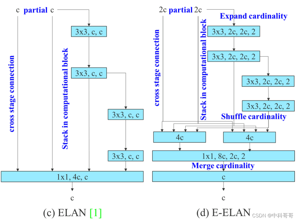
YOLOv7 can obtain more abundant gradient information by putting more gradient flow branches in parallel, and then put the ELAN module, which can lead to higher accuracy and more reasonable delay.

The structure diagram of the C2f module is as follows:

We can easily see that the C2f module is designed with reference to the C3 module and the idea of ​​ELAN, so that YOLOv8 can obtain more abundant gradient flow information while ensuring light weight.

The corresponding Pytorch implementation of the C2f module is as follows:

class C2f(nn.Module):
    # CSP Bottleneck with 2 convolutions
    def __init__(self, c1, c2, n=1, shortcut=False, g=1, e=0.5):  # ch_in, ch_out, number, shortcut, groups, expansion
        super().__init__()
        self.c = int(c2 * e)  # hidden channels
        self.cv1 = Conv(c1, 2 * self.c, 1, 1)
        self.cv2 = Conv((2 + n) * self.c, c2, 1)  # optional act=FReLU(c2)
        self.m = nn.ModuleList(Bottleneck(self.c, self.c, shortcut, g, k=((3, 3), (3, 3)), e=1.0) for _ in range(n))
 
    def forward(self, x):
        y = list(self.cv1(x).split((self.c, self.c), 1))
        y.extend(m(y[-1]) for m in self.m)
        return self.cv2(torch.cat(y, 1))

SPPF improvement

The SPP structure, also known as spatial pyramid pooling, can convert feature maps of any size into feature vectors of fixed size.

Next, let's elaborate on how SPP handles it~

Input layer: first we now have a picture of any size, its size is w * h.

Output layer: 21 neurons – that is, we want to extract 21 features later.

The analysis is shown in the figure below: respectively take the max value in each box in the 1 * 1 block, 2 * 2 block and 4 * 4 sub-picture (that is, take the maximum value in the blue frame), this step is to do Maximum pooling, so that the last extracted eigenvalues ​​(that is, the maximum value taken out) have a total of 1 * 1 + 2 * 2 + 4 * 4 = 21. The obtained features are then concat together.

The structure diagram of SPP in YOLOv5 is shown in the figure below:

In the YOLOv56.0 version, SPPF replaces SPP, and the effect of the two is the same, but the execution time of the former is reduced to 1/2 compared with the latter.

PAN-FPN improvements

The structure diagram of the PAN-FPN part of YOLOv5 and YOLOv6:

The structure diagram of the Neck part of YOLOv5 is as follows:

The structure diagram of the Neck part of YOLOv6 is as follows:

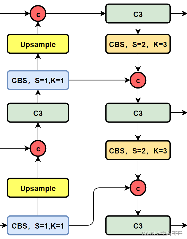
Let's look at the structure diagram of YOLOv8:

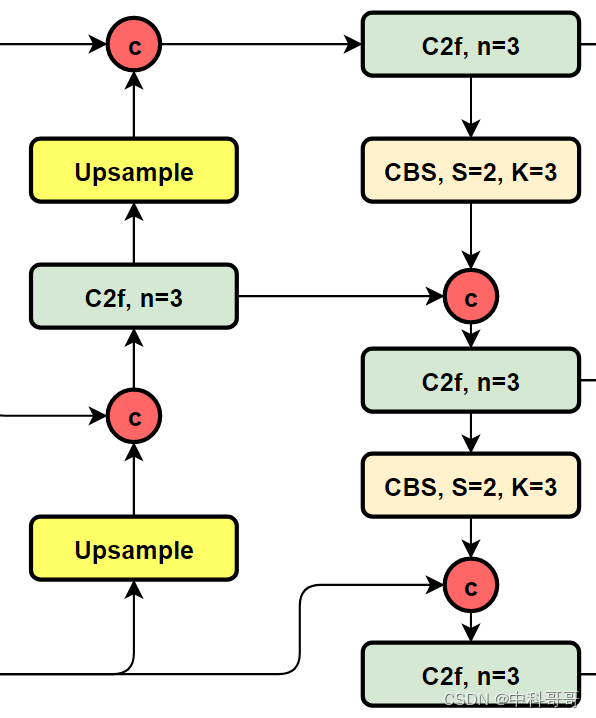
It can be seen that compared with YOLOv5 or YOLOv6, YOLOv8 replaces the C3 module and RepBlock with C2f. At the same time, it can be found carefully that compared with YOLOv5 and YOLOv6, YOLOv8 chooses to remove the 1×1 convolution before upsampling, and different stages of Backbone The output features are directly fed into the upsampling operation.

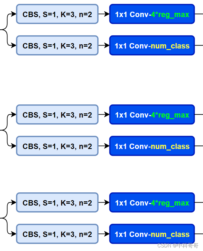
Head section improved

First look at the Head (Coupled-Head) of YOLOv5 itself:

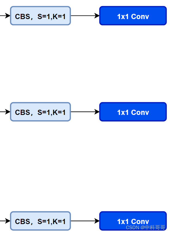
YOLOv8 uses Decoupled-Head, and because of the idea of ​​DFL, the number of channels of the regression head has also become 4*reg_max:

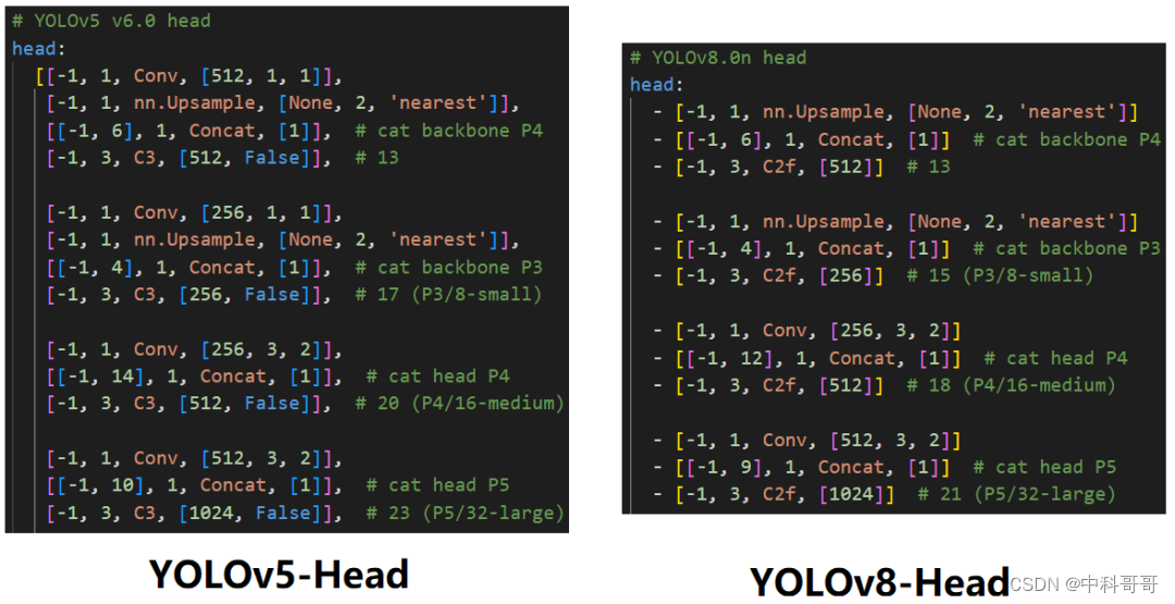
Compare the YAML of YOLOv5 and YOLOv8

Loss function improvements

For YOLOv8, its classification loss is VFL Loss, and its regression loss is in the form of CIOU Loss+DFL, where Reg_max defaults to 16.

The main improvement of VFL is to propose an asymmetric weighting operation, and both FL and QFL are symmetrical. The idea of ​​asymmetric weighting comes from the paper PISA, which pointed out that firstly, the positive and negative samples have an imbalance problem, even in the positive sample, there is also the problem of unequal weight, because the calculation of mAP is the main positive sample.

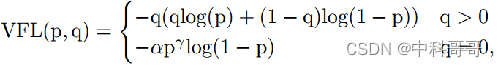
q is the label. When it is a positive sample, q is the IoU of bbox and gt. When it is a negative sample, q=0. When it is a positive sample, FL is not actually used, but ordinary BCE, but there is an additional adaptive IoU weighting for Highlight the master sample. And when it is a negative sample, it is the standard FL. It can be clearly found that VFL is simpler than QFL, and its main features are asymmetric weighting of positive and negative samples, and prominent positive samples as the main samples.

For the DFL (Distribution Focal Loss) here, it mainly models the position of the frame as a general distribution, allowing the network to quickly focus on the distribution of positions close to the target position.

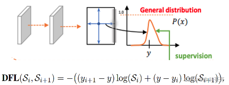
DFL allows the network to focus on values ​​near the target y faster, increasing their probability;

The meaning of DFL is to optimize the probability of the two positions closest to the label y, one left and one right, in the form of cross entropy, so that the network can focus on the distribution of the adjacent area of ​​the target position faster; that is to say, the learned distribution Theoretically, it is near the real floating-point coordinates, and the weight of the distance from the left and right integer coordinates is obtained in the mode of linear interpolation.

sample matching

Label assignment is a very important part of target detection. In the early version of YOLOv5, MaxIOU was used as the label assignment method. However, in practice, it is found that directly using the side length ratio can also achieve the same effect. YOLOv8 abandoned the Anchor-Base method and used the Anchor-Free method, and found a matching method that replaces the side length ratio, TaskAligned.

In order to work with NMS, the anchor assignment of training samples needs to meet the following two rules:

1. Normally aligned Anchor should be able to predict high classification scores while having precise positioning;
2. Misaligned anchors should have low classification scores and be suppressed in the NMS stage. Based on the above two goals, TaskAligned designed a new Anchor alignment metric to measure the level of Task-Alignment at the Anchor level. Moreover, the Alignment metric is integrated in the sample allocation and loss function to dynamically optimize the prediction of each Anchor.

Anchor alignment metric：

The classification score and IoU represent the prediction effect of these two tasks, so TaskAligned uses the high-order combination of classification score and IoU to measure the degree of Task-Alignment. Use the following methods to calculate the Anchor-level alignment for each instance:

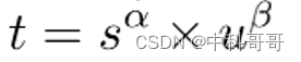
s and u are classification score and IoU value respectively, and α and β are weight hyperparameters. As can be seen from the above formula, t can simultaneously control the classification score and IoU optimization to achieve Task-Alignment, which can guide the network to dynamically focus on high-quality Anchor.

Training sample Assignment：

In order to improve the alignment of the two tasks, TOOD focuses on the Task-Alignment Anchor and uses a simple allocation rule to select training samples: for each instance, select m Anchors with the largest t value as positive samples, and select the remaining Anchor as a negative sample. Then, training is performed by a loss function (a loss function designed for the alignment of classification and localization).

Summarize

Ultralytics released a brand new repository for the YOLO model. It is built as a unified framework for training object detection, instance segmentation, and image classification models.

Here are some key features about the new version:

• User friendly API (command line + Python)
• faster and more accurate
• Support
  Object Detection
  Instance Segmentation
  Image Classification
• Extensible to all previous versions
• new backbone network
• New Anchor-Free head
• new loss function

YOLOv8 also efficiently and flexibly supports multiple export formats, and the model can run on both CPU and GPU.

There are five models in each category of the YOLOv8 model for detection, segmentation and classification. YOLOv8 Nano is the fastest and smallest, while YOLOv8 Extra Large (YOLOv8x) is the most accurate but slowest of them all.

YOLOv8 bundles the following pretrained models:

• Object detection checkpoint trained on the COCO detection dataset with image resolution 640.
• Instance segmentation checkpoint trained on the COCO segmentation dataset with image resolution 640.
• Image classification model pretrained on the ImageNet dataset with image resolution 224.

YOLOv8 test results