Li Mu's "Hands-on Deep Learning" Notes (2) Realizing Linear Regression with Pytorch

For the mathematical basis of linear regression, you can read linear regression here , which is very clear in the book~

It is worth mentioning that the linear regression problem has a global optimal solution

The analytical solution is:

But here the iterative method is used for optimization

Slightly changed the code to realize the visualization of some data

 

Import required packages 

import torch
import matplotlib.pyplot as plt
import numpy as np
from torch.utils import data
from d2l import torch as d2l

The first step is to obtain the dataset

true_w = torch.tensor([2, -3.4])
true_b = torch.tensor(4.2)
features, labels = d2l.synthetic_data(true_w, true_b, 1000)

Synthetic_data function description

Can d2l.synthetic_data also be used here? Or d2l.synthetic_data? ? To query function related information

If you use two question marks, you can view the specific implementation code of the function

help(d2l.synthetic_data)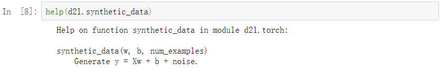

 View input features

print(features.shape)
print(labels.shape)
plt.plot(features[:, 0], features[:, 1], '.')

View the dataset in a 3D coordinate system 

from mpl_toolkits.mplot3d import Axes3D
a = torch.cat([features, labels], axis=1)
fig = plt.figure(figsize=(12, 8))
ax = Axes3D(fig)
ax.scatter(a[:,0], a[:, 1], a[:, 2])

 

The second step is to read the data set and create a data iterator

data_xy = (features, labels)
dataset = data.TensorDataset(*data_xy)
data_iter = data.DataLoader(dataset, batch_size=16, shuffle=True)

The third step is to build the network and initialize the network parameters

from torch import nn
net = nn.Sequential(nn.Linear(2, 1))
net[0].weight.data.normal_(0, 0.02)
net[0].bias.data.fill_(0)

The fourth step is to define the loss function

loss = nn.MSELoss()

The fifth step is to define the optimization algorithm

trainer = torch.optim.SGD(net.parameters(), lr=0.01)

The sixth step, start training

epochs_num = 3
for epoch in range(epochs_num):
    for x, y in data_iter:
        l = loss(net(x), y)
        trainer.zero_grad()
        l.backward()
        trainer.step()
    l = loss(net(features), labels)
    print('epoch:{}, loss:{}'.format(epoch+1, l))

The seventh step is to visualize the training results

fig = plt.figure(figsize=(10, 6))
ax = Axes3D(fig)
ax.scatter(features[0:100, 0], features[0:100, 1], labels[0:100], color='blue')
x = np.linspace(-3, 3, 9)
y = np.linspace(-3, 3, 9)
X, Y = np.meshgrid(x, y)
ax.plot_surface(X=X,
    Y=Y,
    Z=1.9992*X-Y*3.4001+4.1988,
    color='green',
    alpha=0.7
    )
ax.view_init(elev=15,
             azim=10)

The green plane is the result obtained. Due to the large amount of data and few network parameters, after training for three epochs, the plane can fit the original features very well!