Gradient descent algorithm in practice

In the previous article, we explained the mathematical principles of the gradient descent algorithm in detail. To view the mathematical principles of the previous article, please click here . This article mainly uses a simple linear regression to demonstrate the charm of the gradient descent algorithm. Students who don’t understand the principles of the party can also directly code the code, and then look up the information one by one after encountering problems. If you develop in a higher-level direction, then mathematics is definitely indispensable, and you must return to the most basic place. alright! No more nonsense, just go straight to the code!

1. Source of information

The information is compiled by yourself, of course, you can collect the information or download the information yourself, the information is as follows

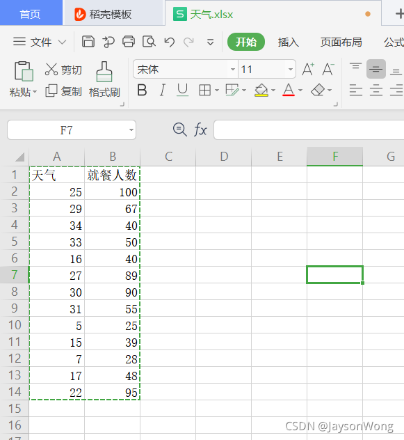
weather	Number of people dining
25	100
29	67
34	40
33	50
16	40
27	89
30	90
31	55
5	25
15	39
7	28
17	48
22	95

The data is in xlsx format and saved in the root directory of the D drive. The data map is as follows:
insert image description here

2. Code

# -*- coding: utf-8 -*-
"""
AUTHOR: jsonwong
TIME: 2021/9/17
"""

import pandas as pd
import numpy as np
import matplotlib.pyplot as plt

def data_process(file_path): # 数据处理函数
    data = pd.read_excel(file_path, header=None, names=['weather', 'number'])
    new_data = data.drop([0])
    new_data.insert(0, 'Ones', 1)
    return new_data

def vectorization(data): # 向量化函数
    cols = data.shape[1]
    X = data.iloc[:, 0:cols-1]  # 取前cols-1列，即输入向量
    y = data.iloc[:, cols-1:cols]  # 取最后一列，即目标向量
    X = np.matrix(X.values)
    y = np.matrix(y.values)
    return X, y

def ComputerCost(X, y, theta): # cost function代价函数
    inner = np.power(((X * theta.T) - y), 2)
    return np.sum(inner) / (2 * len(X))

def gradientDescent(X, y, theta, alpha, epoch): # 梯度下降函数
    temp = np.matrix(np.zeros(theta.shape))  # 初始化一个 θ 临时矩阵(1, 2)
    parameters = int(theta.flatten().shape[1])  # 参数 θ的数量
    cost = np.zeros(epoch)  # 初始化一个ndarray，包含每次epoch的cost
    m = X.shape[0]  # 样本数量m

    for i in range(epoch):
        # 利用向量化一步求解
        temp = theta - (alpha / m) * (X * theta.T - y).T * X
        theta = temp
        cost[i] = ComputerCost(X, y, theta)
    return theta, cost

def visualization(new_data, final_theta, *cost): # 可视化函数
    x = new_data["weather"].values # 横坐标
    # x = np.linspace(new_data.weather.min(), new_data.weather.max(), 6)  # 横坐标
    f = final_theta[0, 0] + (final_theta[0, 1] * x)  # 纵坐标
    plt.plot(x, f, 'r', label='Prediction')
    plt.scatter(new_data.weather, new_data.number, label='Traning Data')
    plt.legend(loc=2)  # 2表示在左上角
    plt.xlabel('weather')
    plt.ylabel('number')
    plt.title('Predicted')
    plt.savefig('D:/predicted')
    plt.show()

def iteration_figure(epoch, cost): # 迭代图像函数
    plt.plot(np.arange(epoch), cost, 'r')
    plt.xlabel('epoch')
    plt.ylabel('cost')
    plt.title('error with epoch')
    plt.savefig('D:/error figure')
    plt.show()

def main():
    file_path = 'D:/天气.xlsx'
    theta = np.matrix([0, 0]) # 初始化theta
    new_data = data_process(file_path)
    X, y = vectorization(new_data)
    final_theta, cost = gradientDescent(X, y, theta, 0.003, 10000)
    visualization(new_data, final_theta)
    iteration_figure(10000, cost)

if __name__ == '__main__':
    main()

3. Results

The linear regression result is as shown in the figure below:
insert image description here
You can use EXCEL to draw the same fitting straight line, as shown in the figure below, you can see that it is almost consistent with our fitted image (inconsistent, need to adjust the number of iterations and learning rate α) The fitting process is as shown in the figure below
insert image description here
: