Machine Learning: gradient descent algorithm theory to explain

background

As the basis for the concept of learning machine learning.

Reprinted from: "gradient descent algorithm theory to explain - machine learning"

1 Overview

Gradient descent (gradient descent) in machine learning in a wide range of applications, whether online or regression Logistic regression, its main purpose is to iteratively find the minimum objective function, or converge to a minimum.
This article from the scene of a downhill start, first put forward the basic idea of gradient descent algorithm, and then explain the principles of the gradient descent algorithm mathematically explain why use gradients, the final realization of a simple example of gradient descent algorithm!

2. gradient descent algorithm

2.1 scenario assumes

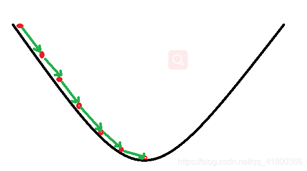
The basic idea of gradient descent method is analogous to a downhill course.
Assume that such a scenario: a man trapped in the mountains, we need to come down the mountain (to find the lowest point of the mountain, which is the valley). But this time a big hill fog, resulting in low visibility; therefore, can not be determined down the path, you must use the information around them step by step to find down the road. This time, we can use gradient descent algorithm to help them down the mountain. How to do it, first of all to his current position as a reference in which to find the steepest place in this position, then take a step toward lowering direction, and then continue with the current position as a reference, find the steepest places, walk until finally reaching the lowest point; empathy mountain, too, but this time it becomes a gradient ascent algorithm

2.2 gradient descent

The basic process of gradient descent down the mountain and on the scene very similar.

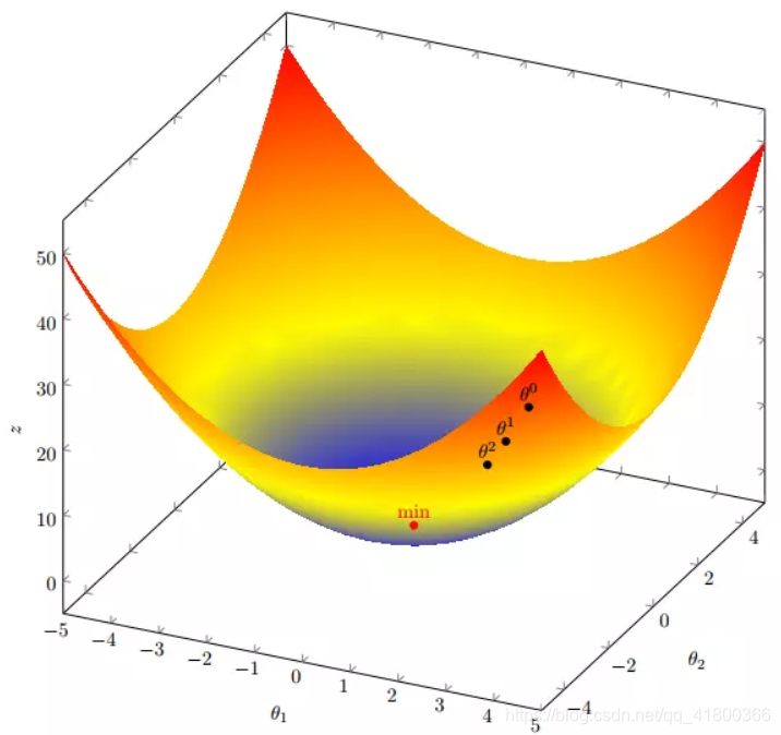
First of all, we have a differentiable function. This function represents the mountain. Our goal is to find the minimum of this function, which is the base of the mountain. The scenario assumes that before, the fastest way is to find the most down a steep current position and direction, and then go down along this direction, corresponding to the function, the point is to find a gradient , and then toward the opposite direction of the gradient, you can make the fastest decline in the value of the function! Because the direction of the gradient is a function of changes in the fastest direction (will explain later)
so we reuse this method, repeatedly strike a gradient, and finally able to reach a local minimum, which is similar to the process we are down. The strike will determine the steepest gradient direction, which is the scene in the direction of the means of measurement. Why then the direction of the gradient is steepest direction? Next, we start with the differential:

2.2.1 differential

Viewing the Significance of differential, you can have a different point of view, the two most common are:

• Image function, the slope of the tangent at a point
• The rate of change of a function
  a few examples of differentiation:

1. Only a single variable differential variable, function

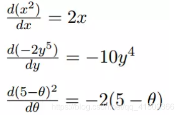
differential 2. multivariable function when a plurality of variables, i.e. separately for each variable differentiating

2.2.2 Gradient

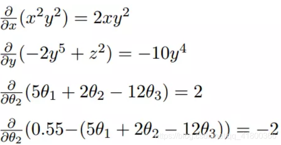
Multivariable generalized gradient is actually a derivative.
The following example:

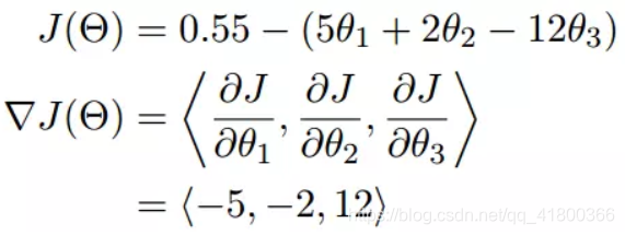
We can see that the gradient is separately for each variable differential, then separated by a comma, the gradient is <> include them, in fact, a gradient vector instructions.

Calculus gradient is a very important concept, previously mentioned meaning gradient

• In univariate function, the gradient is actually a differential function, representing the slope of the tangent function at a given point of
• In multivariable function, the gradient is a vector, the vector has direction, the direction of the gradient pointed to the rise of fixed-point function in the fastest direction

这也就说明了为什么我们需要千方百计的求取梯度！我们需要到达山底，就需要在每一步观测到此时最陡峭的地方，梯度就恰巧告诉了我们这个方向。梯度的方向是函数在给定点上升最快的方向，那么梯度的反方向就是函数在给定点下降最快的方向，这正是我们所需要的。所以我们只要沿着梯度的方向一直走，就能走到局部的最低点！

2.3 数学解释

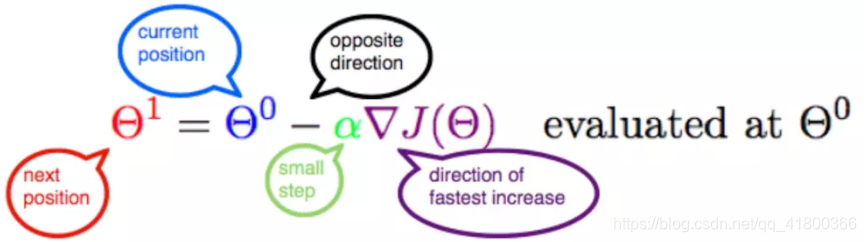
首先给出数学公式：

此公式的意义是：J是关于Θ的一个函数，我们当前所处的位置为Θ0点，要从这个点走到J的最小值点，也就是山底。首先我们先确定前进的方向，也就是梯度的反向，然后走一段距离的步长，也就是α，走完这个段步长，就到达了Θ1这个点！

2.3.1 α

α在梯度下降算法中被称作为学习率或者步长，意味着我们可以通过α来控制每一步走的距离，以保证不要步子跨的太大扯着蛋，哈哈，其实就是不要走太快，错过了最低点。同时也要保证不要走的太慢，导致太阳下山了，还没有走到山下。所以α的选择在梯度下降法中往往是很重要的！α不能太大也不能太小，太小的话，可能导致迟迟走不到最低点，太大的话，会导致错过最低点！

2.3.2 梯度要乘以一个负号

梯度前加一个负号，就意味着朝着梯度相反的方向前进！我们在前文提到，梯度的方向实际就是函数在此点上升最快的方向！而我们需要朝着下降最快的方向走，自然就是负的梯度的方向，所以此处需要加上负号；那么如果时上坡，也就是梯度上升算法，当然就不需要添加负号了。

3. 实例

我们已经基本了解了梯度下降算法的计算过程，那么我们就来看几个梯度下降算法的小实例，首先从单变量的函数开始，然后介绍多变量的函数。

3.1 单变量函数的梯度下降

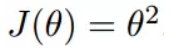
我们假设有一个单变量的函数

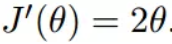
函数的微分，直接求导就可以得到

初始化，也就是起点，起点可以随意的设置，这里设置为1

学习率也可以随意的设置，这里设置为0.4

根据梯度下降的计算公式

我们开始进行梯度下降的迭代计算过程：

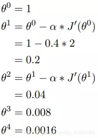
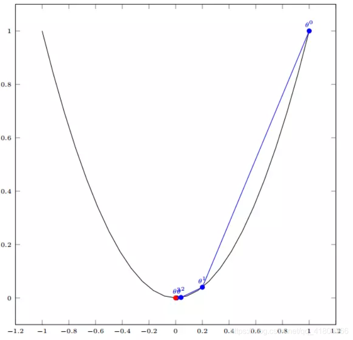
如图，经过四次的运算，也就是走了四步，基本就抵达了函数的最低点，也就是山底

3.2 多变量函数的梯度下降

我们假设有一个目标函数

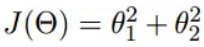
现在要通过梯度下降法计算这个函数的最小值。我们通过观察就能发现最小值其实就是 (0，0)点。但是接下来，我们会从梯度下降算法开始一步步计算到这个最小值！
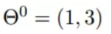
我们假设初始的起点为：

初始的学习率为：

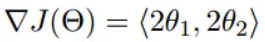
函数的梯度为：

进行多次迭代：

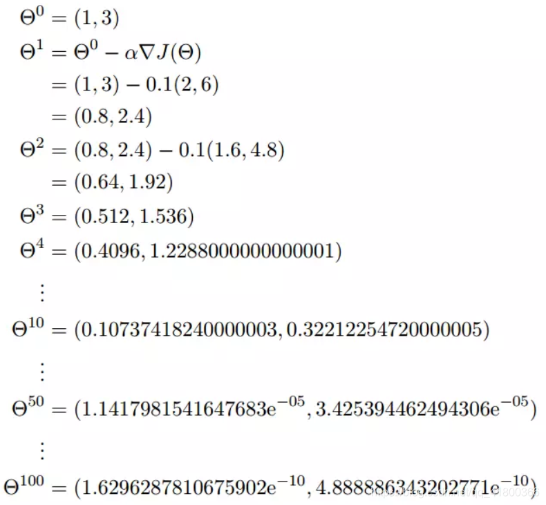
我们发现，已经基本靠近函数的最小值点

4. 代码实现

4. 1 场景分析

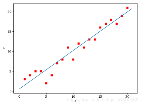
下面我们将用python实现一个简单的梯度下降算法。场景是一个简单的线性回归的例子：假设现在我们有一系列的点，如下图所示：

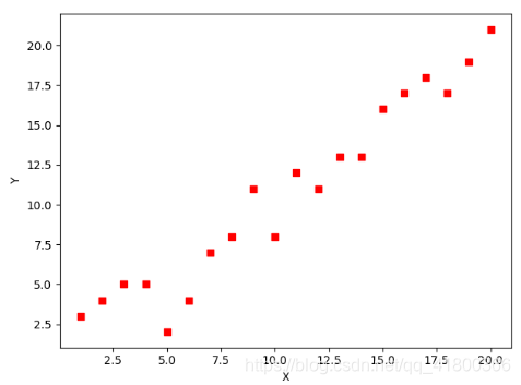
我们将用梯度下降法来拟合出这条直线！

首先，我们需要定义一个代价函数，在此我们选用均方误差代价函数（也称平方误差代价函数）

此公式中

• m是数据集中数据点的个数，也就是样本数
• ½是一个常量，这样是为了在求梯度的时候，二次方乘下来的2就和这里的½抵消了，自然就没有多余的常数系数，方便后续的计算，同时对结果不会有影响
• y 是数据集中每个点的真实y坐标的值，也就是类标签
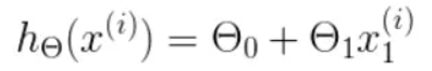
• h 是我们的预测函数（假设函数），根据每一个输入x，根据Θ 计算得到预测的y值，即
  
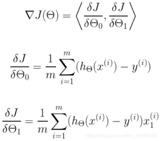
  我们可以根据代价函数看到，代价函数中的变量有两个，所以是一个多变量的梯度下降问题，求解出代价函数的梯度，也就是分别对两个变量进行微分
  
  明确了代价函数和梯度，以及预测的函数形式。我们就可以开始编写代码了。但在这之前，需要说明一点，就是为了方便代码的编写，我们会将所有的公式都转换为矩阵的形式，python中计算矩阵是非常方便的，同时代码也会变得非常的简洁。
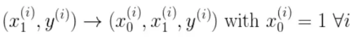
  为了转换为矩阵的计算，我们观察到预测函数的形式
  
  我们有两个变量，为了对这个公式进行矩阵化，我们可以给每一个点x增加一维，这一维的值固定为1，这一维将会乘到Θ0上。这样就方便我们统一矩阵化的计算
  
  然后我们将代价函数和梯度转化为矩阵向量相乘的形式
  

4. 2 代码

首先，我们需要定义数据集和学习率

#!/usr/bin/env python3
# -*- coding: utf-8 -*-
# @Time    : 2019/1/21 21:06
# @Author  : Arrow and Bullet
# @FileName: gradient_descent.py
# @Software: PyCharm
# @Blog    ：https://blog.csdn.net/qq_41800366

from numpy import *

# 数据集大小 即20个数据点
m = 20
# x的坐标以及对应的矩阵
X0 = ones((m, 1))  # 生成一个m行1列的向量，也就是x0，全是1
X1 = arange(1, m+1).reshape(m, 1)  # 生成一个m行1列的向量，也就是x1，从1到m
X = hstack((X0, X1))  # 按照列堆叠形成数组，其实就是样本数据
# 对应的y坐标
y = np.array([
    3, 4, 5, 5, 2, 4, 7, 8, 11, 8, 12,
    11, 13, 13, 16, 17, 18, 17, 19, 21
]).reshape(m, 1)
# 学习率
alpha = 0.01
1234567891011121314151617181920212223

接下来我们以矩阵向量的形式定义代价函数和代价函数的梯度

# 定义代价函数
def cost_function(theta, X, Y):
    diff = dot(X, theta) - Y  # dot() 数组需要像矩阵那样相乘，就需要用到dot()
    return (1/(2*m)) * dot(diff.transpose(), diff)


# 定义代价函数对应的梯度函数
def gradient_function(theta, X, Y):
    diff = dot(X, theta) - Y
    return (1/m) * dot(X.transpose(), diff)
12345678910

最后就是算法的核心部分，梯度下降迭代计算

# 梯度下降迭代
def gradient_descent(X, Y, alpha):
    theta = array([1, 1]).reshape(2, 1)
    gradient = gradient_function(theta, X, Y)
    while not all(abs(gradient) <= 1e-5):
        theta = theta - alpha * gradient
        gradient = gradient_function(theta, X, Y)
    return theta


optimal = gradient_descent(X, Y, alpha)
print('optimal:', optimal)
print('cost function:', cost_function(optimal, X, Y)[0][0])
12345678910111213

当梯度小于1e-5时，说明已经进入了比较平滑的状态，类似于山谷的状态，这时候再继续迭代效果也不大了，所以这个时候可以退出循环！
运行代码，计算得到的结果如下：

print('optimal:', optimal)  # 结果 [[0.51583286][0.96992163]]
print('cost function:', cost_function(optimal, X, Y)[0][0])  # 1.014962406233101
12

通过matplotlib画出图像，

# 根据数据画出对应的图像
def plot(X, Y, theta):
    import matplotlib.pyplot as plt
    ax = plt.subplot(111)  # 这是我改的
    ax.scatter(X, Y, s=30, c="red", marker="s")
    plt.xlabel("X")
    plt.ylabel("Y")
    x = arange(0, 21, 0.2)  # x的范围
    y = theta[0] + theta[1]*x
    ax.plot(x, y)
    plt.show()


plot(X1, Y, optimal)
1234567891011121314

所拟合出的直线如下

全部代码如下，大家有兴趣的可以复制下来跑一下看一下结果：

#!/usr/bin/env python3
# -*- coding: utf-8 -*-
# @Time    : 2019/1/21 21:06
# @Author  : Arrow and Bullet
# @FileName: gradient_descent.py
# @Software: PyCharm
# @Blog    ：https://blog.csdn.net/qq_41800366

from numpy import *

# 数据集大小 即20个数据点
m = 20
# x的坐标以及对应的矩阵
X0 = ones((m, 1))  # 生成一个m行1列的向量，也就是x0，全是1
X1 = arange(1, m+1).reshape(m, 1)  # 生成一个m行1列的向量，也就是x1，从1到m
X = hstack((X0, X1))  # 按照列堆叠形成数组，其实就是样本数据
# 对应的y坐标
Y = array([
    3, 4, 5, 5, 2, 4, 7, 8, 11, 8, 12,
    11, 13, 13, 16, 17, 18, 17, 19, 21
]).reshape(m, 1)
# 学习率
alpha = 0.01


# 定义代价函数
def cost_function(theta, X, Y):
    diff = dot(X, theta) - Y  # dot() 数组需要像矩阵那样相乘，就需要用到dot()
    return (1/(2*m)) * dot(diff.transpose(), diff)


# 定义代价函数对应的梯度函数
def gradient_function(theta, X, Y):
    diff = dot(X, theta) - Y
    return (1/m) * dot(X.transpose(), diff)


# 梯度下降迭代
def gradient_descent(X, Y, alpha):
    theta = array([1, 1]).reshape(2, 1)
    gradient = gradient_function(theta, X, Y)
    while not all(abs(gradient) <= 1e-5):
        theta = theta - alpha * gradient
        gradient = gradient_function(theta, X, Y)
    return theta


optimal = gradient_descent(X, Y, alpha)
print('optimal:', optimal)
print('cost function:', cost_function(optimal, X, Y)[0][0])


# 根据数据画出对应的图像
def plot(X, Y, theta):
    import matplotlib.pyplot as plt
    ax = plt.subplot(111)  # 这是我改的
    ax.scatter(X, Y, s=30, c="red", marker="s")
    plt.xlabel("X")
    plt.ylabel("Y")
    x = arange(0, 21, 0.2)  # x的范围
    y = theta[0] + theta[1]*x
    ax.plot(x, y)
    plt.show()


plot(X1, Y, optimal)
123456789101112131415161718192021222324252627282930313233343536373839404142434445464748495051525354555657585960616263646566

5. 小结

At this point, it basically introduced over gradient descent algorithm of the basic ideas and processes, and with python implements a simple case of gradient descent algorithm to fit a straight line!
Finally, we return to the scene at the beginning of the article proposed hypothesis:
this down people actually represents the back-propagation algorithm , down the path actually represents the algorithm had been looking for parameters Θ, the steepest mountain current point direction is actually the cost function at this point in the direction of the gradient, the scene observation tool used by the steepest direction is differential . Time before the next observation is that we have the learning rate α algorithm defined.
We can see scenes assumptions and gradient descent algorithm corresponding well done!

Most of the contents of this article from a senior, so thanks for sharing! Thank you!