Operating system 9: continuous allocation and swap of storage management

In order to load the user program into memory, a certain amount of memory space must be allocated for it. The continuous allocation method is the earliest memory allocation method, which was widely used in the OS in the 1960s and 1980s. This allocation method allocates a continuous memory space for a user program, that is, the logic of the code or data in the program. The address is adjacent, which is reflected in the adjacent physical address when the memory space is allocated . Continuous allocation methods can be divided into four categories: single continuous allocation , fixed partition allocation , dynamic partition allocation , and dynamic relocatable partition allocation algorithms.

(1) Single continuous allocation

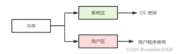
In the single-program environment, the memory management method at that time was to divide the memory into two parts, the system area and the user area . The system area was only provided for the OS, and it was usually placed in the low-address part of the memory. In the user area memory, only one user program is installed, that is, the user space of the entire memory is exclusively occupied by this program. Such a memory allocation method is called a single contiguous allocation method.

Although many of the early single-user and single-task operating systems were equipped with memory protection mechanisms to prevent user programs from damaging the operating system, several common single-user operations produced in the 1980s In the system, such as CP/M, MS-DOS and RT11, etc., no memory protection measures are taken. This is because, on the one hand, hardware can be saved, and on the other hand, in a single-user environment, the machine is exclusively occupied by one user, and there is no possibility of interference from other users, so this is feasible. Even if there is a destructive behavior, it will only be that the user program itself destroys the operating system, and its consequences are not serious, it will only affect the operation of the user program, and the operating system is easy to reload the memory by restarting the system.

(2) Fixed partition allocation

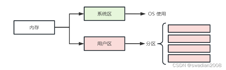
In order to load multiple programs in the memory without interfering with each other, the entire user space is divided into several fixed-size areas, and only one job is loaded in each partition . This forms the earliest and simplest partitioned storage management method that can run multi-programs . If there are four user partitions in memory, four programs are allowed to run concurrently. When there is an idle partition, a job of an appropriate size can be selected from the backup job queue of the external storage and loaded into the partition. When the job ends, another job can be found from the backup job queue and transferred to the partition.

2.1 - Method of partitioning

The user space of memory can be divided into several fixed-size partitions in the following two ways:

Partitions are of equal size (meaning that all memory partitions are of equal size). Its disadvantage is the lack of flexibility, that is, when the program is too small, it will cause waste of memory space. When the program is too large, one partition is not enough to load the program, so the program cannot run. However, for the occasion of using one computer to control multiple identical objects at the same time, because the memory space required by these objects is often the same size, this division method is more convenient and practical, so it is widely used. For example, the furnace temperature group control system uses one computer to control multiple identical smelting furnaces.
Partition sizes vary . In order to increase the flexibility of memory allocation, the memory partition should be divided into several partitions of different sizes. It is best to investigate the size of the jobs that are often run on the system and divide them according to the needs of the users. Generally, the memory area can be divided into multiple smaller partitions, a moderate amount of medium partitions, and a small number of large partitions, so that appropriate partitions can be allocated according to the size of the program.

2.2 - Memory allocation

In order to facilitate memory allocation, partitions are usually queued according to their size, and a partition usage table is established for it , where each entry includes the starting address, size and status (allocated or not) of each partition. When a user program is to be loaded, the memory allocation program searches the table according to the size of the user program, finds an unallocated partition that can meet the requirements, allocates it to the program, and then assigns it to the program. The status is set to "allocated". If no partition of sufficient size is found, memory allocation for the user program is refused. //Use the partition table to maintain the partition status

Fixed partition allocation is the earliest storage management method that can be used in multiprogramming systems. Since the size of each partition is fixed, it will inevitably cause waste of storage space, so it is rarely used in general-purpose OS . However, in some control systems used to control multiple identical objects, since the control program of each object has the same size and has been compiled in advance, the required data is also certain, so fixed partition storage management is still used Way. //There is a problem of memory waste in the fixed partition allocation method

(3) Dynamic partition allocation

Dynamic partition allocation, also known as variable partition allocation, dynamically allocates memory space for a process according to its actual needs . When implementing dynamic partition allocation, three aspects will be involved : the data structure used in partition allocation , the partition allocation algorithm , and the allocation and recovery operations of partitions .

3.1 - Data structures in dynamic partition allocation

In order to realize dynamic partition allocation, corresponding data structures must be configured in the system to describe the situation of free partitions and allocated partitions , and provide basis for allocation. The commonly used data structures have the following two forms:

Free partition table. Set up a free partition table in the system to record the situation of each free partition . Each free partition occupies an entry, which includes data items such as partition number, partition size, and partition start address.

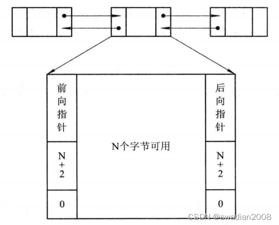
Free partition chain . In order to realize the allocation and linking of free partitions, some information for controlling partition allocation and forward pointers for linking the partitions are set at the beginning of each partition, and a backward pointer is set at the end of the partitions. Through forward and backward link pointers, all free partitions can be linked into a two-way link. For the convenience of retrieval, the status bit and partition size entry are repeatedly set at the end of the partition. After the partition is allocated, change the status bit from "0" to "1" . At this time, the forward and backward pointers are meaningless. //Manage partitions through linked list

3.2 - Dynamic Partition Allocation Algorithm

In order to load a new job into memory, a partition must be selected from the free partition table or free partition chain to assign to the job according to a certain allocation algorithm. // The memory allocation algorithm has a great impact on system performance, which will be introduced in detail later

3.3 - Partition allocation operations

In the dynamic partition storage management method, the main operation is to allocate memory and reclaim memory .

Allocate memory

The system should use some sort of allocation algorithm to find a partition of the required size from the free partition chain (table).

Let the requested partition size be u.size, and the size of each free partition in the table can be expressed as m.size. If m.size - u.size <= size (size is the pre-specified size of the remaining partition that will not be cut), it means that the excess part is too small, and the partition can be allocated to the requester without further cutting. //When the partition can no longer be split, allocate the entire partition

Otherwise (that is, the excess part exceeds the size), a piece of memory space is allocated from the partition according to the requested size, and the remaining part remains in the free partition chain (table). Then, return the first address of the allocated area to the caller.

reclaim memory

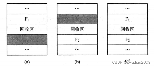
When the process finishes running and releases the memory, the system finds the corresponding insertion point from the free area chain (table) according to the first address of the reclaimed area . At this time, one of the following four situations may occur: //Recycling operation is to regenerate the free memory The process of putting back the free partition table

The reclaimed area is adjacent to the previous free partition F1 of the insertion point. At this time, the reclaimed area should be merged with the previous partition of the insertion point. There is no need to allocate new entries for the reclaimed partition, but only to modify the size of its previous partition F1.
The reclaimed partition is adjacent to the next free partition F2 at the insertion point. At this time, the two partitions can also be merged to form a new free partition, but the first address of the reclaimed area is used as the first address of the new free area, and the size is the sum of the two.
The recovery area is adjacent to the two partitions before and after the insertion point at the same time. At this time, the three partitions are combined to use the entry of F1 and the first address of F1, and the entry of F2 is canceled, and the size is the sum of the three.
The recycling area is neither adjacent to F1 nor to F2. At this time , a new entry should be created separately for the recovery area , fill in the first address and size of the recovery area, and insert it into the appropriate position in the free chain according to the first address.

(4) Dynamic partition allocation algorithm based on sequential search

In order to realize dynamic partition allocation, usually the free partitions in the system are linked into a chain. The so-called sequential search refers to sequentially searching the free partitions on the free partition chain to find a partition whose size can meet the requirements . There are four kinds of dynamic partition allocation algorithms based on sequential search: first-fit algorithm , cycle first-fit algorithm , best-fit algorithm and worst-fit algorithm . //Suitable for systems with not many partitions

4.1 - First fit (FF) algorithm

The FF algorithm requires that the chain of free partitions be linked in order of increasing address . When allocating memory, search sequentially from the beginning of the chain until a free partition with a size that meets the requirements is found . Then according to the size of the job, a memory space is allocated from the partition and allocated to the requester, and the remaining free partitions remain in the free chain. If a partition that can meet the requirements cannot be found from the beginning of the chain to the end of the chain, it indicates that there is not enough memory in the system to allocate to the process, memory allocation fails and returns.

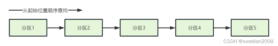
The algorithm tends to preferentially utilize the free partitions in the low-address part of the memory , thereby reserving a large free area in the high-address part. This creates conditions for large memory allocations for large jobs that arrive later. Its disadvantage is that the low-address part is continuously divided, and many small free partitions that are difficult to use will be left, which are called fragments. And each search starts from the low-address part, which undoubtedly increases the overhead when searching for available free partitions.

4.2 - Cyclic first fit (next fit, NF) algorithm

In order to avoid leaving many small free partitions in the low-address part and reduce the overhead of finding available free partitions, when the loop first adaptation algorithm allocates memory space for a process, it no longer searches from the beginning of the chain every time, but starts from the The next free partition of the free partition found last time starts searching until a free partition that meets the requirements is found, and a memory space equal to the requested size is allocated from it to the job.

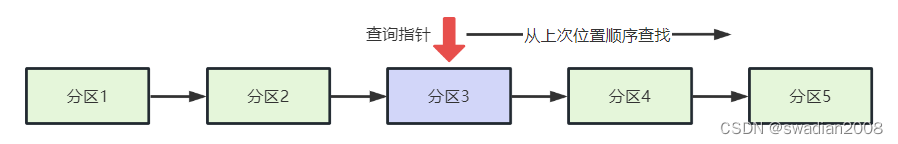
In order to realize this algorithm, an initial search pointer should be set to indicate the free partition for the next initial search, and a circular search method should be used, that is, if the size of the last (chain tail) free partition still cannot meet the requirements, it should return Go to the first free partition and compare whether its size meets the requirements. Once found, the starting seek pointer should be adjusted. This algorithm can make the free partitions in the memory more evenly distributed, thereby reducing the overhead of finding free partitions , but this will lack large free partitions.

4.3 - Best fit (BF) algorithm

The so-called "best" means that every time memory is allocated for a job, the smallest free partition that can meet the requirements is always allocated to the job, so as to avoid "overkill and underutilization". In order to speed up the search, the algorithm requires all free partitions to form a chain of free partitions in ascending order according to their capacities . In this way, the free area that can meet the requirements found for the first time must be the best.

In isolation, the best fit algorithm seems to be the best, but not necessarily in the macro. Because the remaining part cut off after each allocation is always the smallest, in this way, many fragments that are difficult to use will be left in the memory .

4.4 - Worst fit (WF) algorithm

Because the worst-fit allocation algorithm selects free partitions, it is just the opposite of the best-fit algorithm: when scanning the entire free partition table or linked list, it always selects the largest free area, and divides a part of the storage space for the job to use. There is a lack of large free partitions, so it is called the worst-fit algorithm.

In fact, such an algorithm may not be the worst. Its advantage is that the remaining free area will not be too small, and the possibility of fragmentation is the smallest , which is beneficial to medium and small jobs. At the same time, the search efficiency of the worst-fit allocation algorithm is very high . This algorithm requires that all free partitions be formed into a chain of free partitions in descending order according to their capacity. When searching, it is only necessary to check whether the first partition can satisfy As required by the job.

(5) Dynamic partition allocation algorithm based on index search

The dynamic partition allocation algorithm based on sequential search is more suitable for systems that are not too large. When the system is very large, there may be many memory partitions in the system, and the corresponding free partition chain may be very long. At this time, the sequential search partition method may be very slow. In order to improve the speed of searching for free partitions , dynamic partition allocation algorithms based on index search are often used in large and medium-sized systems. At present, the commonly used ones are fast adaptation algorithm , buddy system and hash algorithm .

5.1 - Quick fit algorithm

This algorithm is also called classification search method. It classifies free partitions according to their capacity. For all free partitions with the same capacity in each category, a separate list of free partitions is established, so that there are multiple free partition lists in the system . At the same time, a management index table is set up in the memory, and each index entry corresponds to a type of free partition, and records the pointer of the head of the linked list of free partitions of this type. //Like a hash table

The classification of free partitions is based on the space commonly used by processes, such as 2KB, 4KB, 8KB, etc. For partitions of other sizes, free partitions such as 7KB can be placed in either an 8KB linked list or a special in the linked list of free areas.

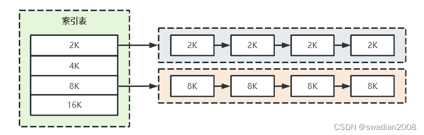
The algorithm is divided into two steps when searching for free partitions that can be allocated:

The first step is to find the smallest free area linked list that can accommodate it from the index table according to the length of the process;
The second step is to remove the first block from the linked list and allocate it.

In addition, when the algorithm allocates free partitions, it will not split any partitions, so large partitions can be reserved to meet the demand for large space, and memory fragmentation will not be generated. The advantage is that the search efficiency is high .

The main disadvantage of this algorithm is that in order to effectively merge partitions, the algorithm is complicated when the partitions are returned to the main memory, and the system overhead is relatively large . In addition, when the algorithm allocates free partitions, it uses processes as units, and a partition belongs to only one process, so there is more or less waste in a partition allocated to a process. This is a typical practice of exchanging space for time .

5.2 - The buddy system

The algorithm stipulates that no matter the allocated partition or the free partition, its size is 2 to the power of k (k is an integer). Assuming that the available space capacity of the system is 2^m words, when the system starts running, the entire memory area is a free partition with a size of 2^m.

During the running of the system, due to continuous division, several discontinuous free partitions will be formed, and these free partitions are classified according to the size of the partitions. For all free partitions with the same size, a free partition doubly-linked list is separately set up, so that free partitions of different sizes form k free partition linked lists. // One allocation requires multiple splits

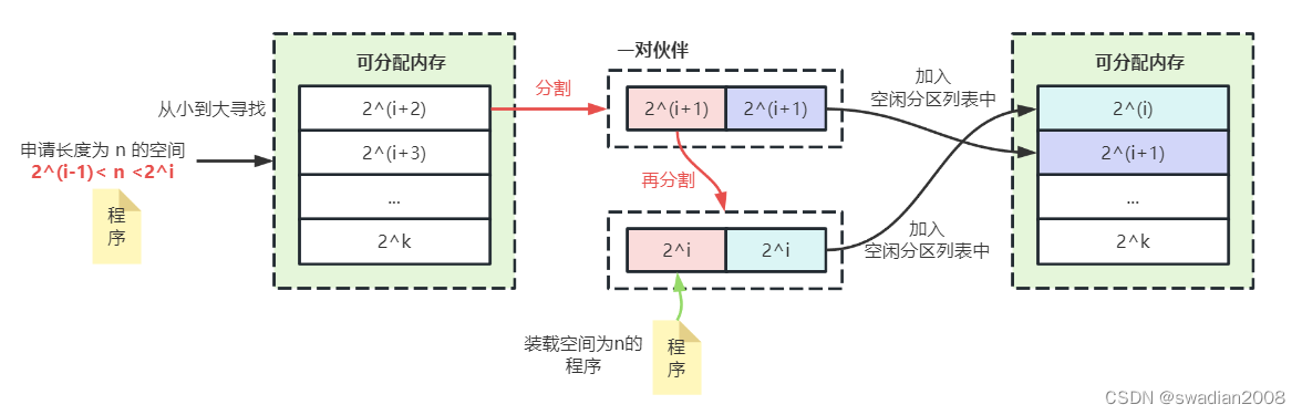
When it is necessary to allocate a storage space with a length of n for a process, first calculate an i value so that 2^(i-1) < n <= 2^i, and then in the free partition list with a free partition size of 2^i find.

If found, the free partition is assigned to the process. Otherwise, it indicates that the free partitions with a length of 2^i have been exhausted, and then search in the free partition list with a partition size of 2^(i+1). If there is a free partition of 2^(i+1), divide the free partition into two equal partitions . These two partitions are called a pair of partners. One of the partitions is used for allocation, and the other is added In the list of free partitions whose partition size is 2^i.

If there is no free partition with a size of 2^(i+1), it is necessary to search for a free partition with a size of 2^(i+2). If it is found, it will be divided twice: first, divide it Divided into two partitions with a size of 2^(i+1), one is used for allocation, and one is added to the list of free partitions with a size of 2^(i+1); the second time, the first time is used for allocation The free area of the partition is divided into two partitions of 2^i, one is used for allocation, and the other is added to the linked list of free partitions with a size of 2^i.

If still not found, continue to search for free partitions with a size of 2^(i+3), and so on. It can be seen that, in the worst case, it may be necessary to divide 2^k free partitions k times to obtain the required partitions.

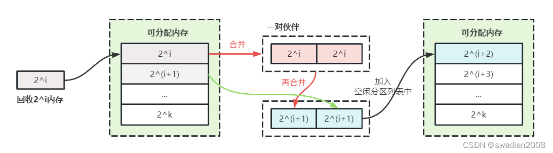
Just as one allocation may require multiple splits, one recovery may also require multiple merges . For example, when reclaiming a free partition with a size of 2^i, if there is a free partition of 2i in advance, it should be merged with the partner partition It is a free partition with a size of 2^(i+1). If there is a free partition with a size of 2^(i+1), it should continue to be merged with its partner partition into a free partition with a size of 2^(i+2). So on and so forth. //If there are pairs of identical free partitions, merge them

In the partner system, the time performance of its allocation and reclamation depends on the time spent in finding the location of free partitions and splitting and merging free partitions. When reclaiming free partitions, free partitions need to be merged, so its time performance is worse than the fast adaptation algorithm, but because it uses the index search algorithm, it is better than the sequential search algorithm. As for its space performance, because the idle partitions are merged, the small idle partitions are reduced, and the usability of the idle partitions is improved , so it is better than the fast adaptation algorithm, and slightly worse than the sequential search method.

5.3 - Hash Algorithms

In the above classification search algorithm and buddy system algorithm, the free partitions are classified according to the size of the partitions. For each type of free partitions with the same size, a free partition list is established separately. When allocating space for a process, it is necessary to find the entry corresponding to the size of the required space in a management index table, and obtain the corresponding head pointer of the linked list of free partitions, so as to obtain a free partition by searching. If the idle partitions are classified more finely, there will be more entries in the corresponding index table, so the time spent searching for the entries in the index table will be significantly increased.

The hash algorithm is to use the advantages of fast hash search and the distribution of free partitions in the available free area table to establish a hash function and construct a hash table with the size of the free partition as the key. An entry records a corresponding head pointer of the linked list of free partitions. //Reduce the time overhead of searching the entries of the index table

When allocating free partitions, according to the size of the required free partitions, the position in the hash table is obtained through hash function calculation, and the corresponding free partition linked list is obtained from it to realize the optimal allocation strategy.

(6) Dynamic relocatable area allocation

6.1 - Compact

An important feature of the continuous allocation method is that a system or user program must be loaded into a contiguous memory space . When a computer runs for a period of time, its memory space will be divided into many small partitions, and there is no large free space. Even if the sum of the capacity of many scattered small partitions is greater than the program to be loaded, the program cannot be loaded into the memory because these partitions are not adjacent . //Because there are too many fragments and cannot be continuous, memory is wasted

For example, there are four non-adjacent small partitions in the memory, their capacities are 10 KB, 30 KB, 14 KB and 26 KB respectively, and their total capacity is 80 KB, but if a job arrives now, it is required to obtain 40 KB of memory space for which the job cannot be loaded because a contiguous space must be allocated. This kind of small partition that cannot be used is the "fragment" mentioned above , or "fraction" .

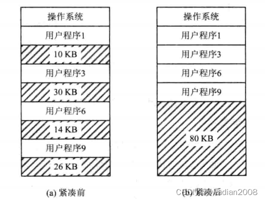
One way to load large jobs is to move all the jobs in memory so that they are all adjacent . In this way, multiple idle small partitions that were originally dispersed can be spliced into one large partition, and a job can be loaded into this partition. This method of splicing multiple scattered small partitions into one large partition by moving the position of the job in the memory is called "splicing" or "compacting".

Although "compact" can obtain a large free space, it also brings new problems. After each "compact", the moved program or data must be relocated . In order to improve the utilization of memory, the system often needs to be "compacted" during operation. Every time "compacted", the address of the moved program or data must be modified, which is not only a very troublesome thing , but also greatly affects the efficiency of the system. Then, using the dynamic relocation method will be able to solve this problem well .

6.2 - Dynamic relocation

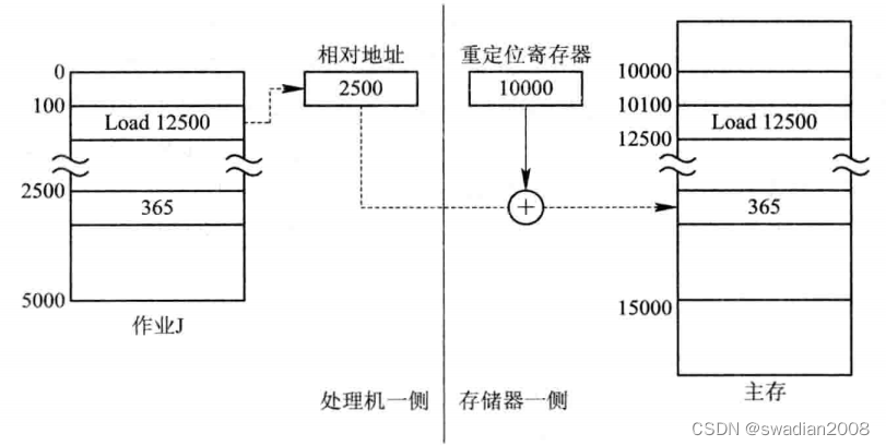
In the method of dynamic runtime loading, all addresses after the job is loaded into memory are still relative (logical) addresses. Instead, the work of converting relative addresses to absolute (physical) addresses is deferred until the program instructions are actually executed.

In order to make the address conversion not affect the execution speed of the instruction, there must be the support of the hardware address conversion mechanism, that is, a relocation register must be added in the system to store the starting address of the program (data) in the memory. When the program is executed, the actually accessed memory address is formed by adding the relative address and the address in the relocation register . //relative address + relocation register address

The address translation process is automatically performed with each instruction or data access during program execution, so it is called dynamic relocation . When the system "compacts" the memory and moves several programs from one part of the memory to another, there is no need to make any changes to the programs, just use the new starting address of the program in the memory to replace the original starting address. start address. //The realization principle of dynamic relocation

6.3 - Dynamic Relocation Partition Allocation Algorithm

The dynamic relocation partition allocation algorithm is basically the same as the dynamic partition allocation algorithm, the only difference is that in this allocation algorithm, a compact function is added .

Usually, when the algorithm cannot find a large enough free partition to meet the user's needs, if the sum of the capacity of all small free partitions is greater than the user's request, then the memory must be "compacted", and the "compact" The resulting large free partitions are allocated to users. If the sum of the capacities of all the small free partitions is still smaller than the user's requirement, the allocation failure information will be returned. //If the memory is not enough, trigger a compaction, the memory recovery of the Java virtual machine is this principle

2. Swapping

Swap technology, also known as swap technology, was first used in CTSS, a single-user time-sharing system of the Massachusetts Institute of Technology. Since the memory of the computer was very small at that time, the swap technology was introduced in order to enable the system to run multiple user programs in a time-sharing manner . The system stores all user jobs on the disk, and only one job can be loaded into the memory at a time. When a time slice of the job is used up, it is transferred to the backup queue of the external memory to wait, and then it is transferred from the backup queue. Load another job into memory. This is the swap technique used in the earliest time-sharing systems. It is rarely used now.

It can be seen from the above that to realize the swap between internal and external memory, there must be an external memory with high I/O speed in the system, and its capacity must be large enough to accommodate all users who are running time-sharing Jobs, currently the most commonly used is large-capacity disk storage.

(1) Swap technology in multi-programming environment

1.1 - Introduction of swaps

In a multi-programming environment, on the one hand, some processes in the memory are blocked because an event has not occurred, but it takes up a large amount of memory space, and sometimes even all processes in the memory are blocked. And there is no runnable process, forcing the CPU to stop and wait; on the other hand, there are many jobs, because the memory space is insufficient, they have been resident in the external memory, and cannot enter the memory to run. Obviously, this is a serious waste of system resources and reduces system throughput.

In order to solve this problem, a swap (also known as an exchange) facility has been added to the system. The so-called "swapping" refers to swapping out the temporarily inoperable processes or temporarily unused programs and data in the memory to the external memory in order to free up enough memory space, and then the processes or processes that are already capable of running Programs and data are swapped into memory . Swap is an effective measure to improve memory utilization, which can directly improve processor utilization and system throughput. //Increase resource utilization

1.2 - Types of swaps

At each swap, a certain amount of programs or data are swapped into or out of memory. According to the quantity swapped at each swap, swaps can be divided into the following two categories:

Whole swap . The mid-level scheduling of the processor is actually the swap function of the memory, and its purpose is to solve the problem of memory shortage, and further improve the utilization rate of the memory and the throughput of the system. Since the swap is , it is called "process swap" or "whole swap". This swap is widely used in multiprogramming systems and as an intermediate processor scheduling.
Page (segment) swapping . If the swap is performed in units of a "page" or "segment" of the process, it is called "page swap" or "segment swap" respectively, and collectively referred to as "partial swap". This swapping approach is the basis for on-demand paging and on-demand fragmentation storage management, which is intended to support virtual storage systems . //Page swap, introduced in paging and segmentation

In order to realize process swap, the system must be able to realize three functions: management of swap space , process swap out and process swap in .

(2) Management of swap space

2.1 - The main goal of swap space management

In an OS with a swap function, the disk space is usually divided into two parts, the file area and the swap area .

Main Objectives of File Area Management

The file area takes up most of the disk space and is used to store various files. Since the usual files reside on the external storage for a long time, the frequency of access to them is low, so the main goal of file area management is to improve the utilization of file storage space , and then to improve file access. access speed. Therefore, a discrete allocation method is adopted for the management of the file area space . //Give priority to space, followed by speed

The main goal of swap space management

Swap space occupies only a small portion of disk space and is used to store processes swapped out of memory. Since these processes reside in the swap area for a short period of time, and the frequency of swap operations is high, the main goal of swap space management is to increase the speed of process swapping in and out, and then Improve the utilization of file storage space. For this reason, the continuous allocation method is adopted for the management of the swap area space , and the fragmentation problem in the external storage is less considered. //Give priority to speed, followed by space

2.2 - Data structure in the management of free disk blocks in the swap area

In order to realize the management of the free disk blocks in the swap area, a corresponding data structure should be configured in the system to record the usage of the free disk blocks in the swap area of the external storage . The form of its data structure is similar to the data structure used in the dynamic partition allocation method of memory, that is, the free partition table or free partition chain can also be used . Each entry in the free partition table should contain two items: the first address of the swap area and its size , which are represented by the disk block number and the number of disk blocks respectively.

2.3 - Allocation and recovery of swap space

Since the allocation of the swap partition adopts the continuous allocation method, the allocation and recovery of the swap space are similar to the memory allocation and recovery methods in the dynamic partition mode . The allocation algorithm can be the first-fit algorithm, the cycle first-fit algorithm, or the best-fit algorithm.

(3) Process swap out and swap in

When the kernel finds that there is insufficient memory due to an operation, for example, when a process needs more memory space due to the creation of a child process, but there is not enough memory space, etc., it calls the swap process , its main The task is to implement process swapping out and swapping in . //The swap operation is implemented by a specific process

3.1 - Process swapping out

When swapping processes out, some processes in the memory are called out to the swap area to free up memory space. The swap out process can be divided into the following two steps:

(1) Select the process to be swapped out. When the swap process selects the process to be swapped out, it will check all the processes residing in the memory, and select the process in the blocked state or sleeping state first . When there are multiple such processes, the process with the lowest priority should be selected as a swap out process. In some systems, in order to prevent low-priority processes from being swapped out soon after being transferred into memory, it is also necessary to consider the residence time of the process in memory. If there is no blocking process in the system, but the current memory space is still not enough to meet the needs, the ready process with the lowest priority is selected to be swapped out.

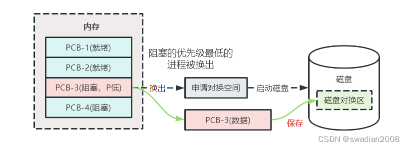
(2) The process swaps out the process. It should be noted that after choosing to swap out a process, only non-shared programs and data segments can be swapped out when the process is swapped out , and those shared programs and data segments cannot be swapped out as long as there are processes that need it. out. When swapping out, you should apply for the swap space first , and if the application is successful, start the disk, and transfer the program and data of the process to the swap area of the disk. If there is no error in the transmission process, the memory space occupied by the process can be reclaimed, and data structures such as the process control block and the memory allocation table of the process can be modified accordingly. If there are still processes that can be swapped out in the memory at this time, the swapping process will continue until there is no more blocked process in the memory.

3.2 - Process swapping

The swap process will perform the swap-in operation at regular intervals. It first looks at the status of all the processes in the PCB collection, and finds the processes that are in the "ready" state but have been swapped out . When there are many such processes, it will select the process that has been swapped out to the disk for the longest time (must be greater than the specified time, such as 2s) as the swap-in process and apply for memory for it. If the application is successful, the process can be directly transferred from the external storage to the internal memory; if it fails, some processes in the memory need to be swapped out to free up enough memory space, and then the process can be transferred in.

After the swapping process is successfully swapped into a process, if there are still processes that can be swapped in, then continue to execute the swapping in and swapping out process, and the rest of the processes in the "ready and swapped out" state are swapped in one after another until they are in the memory. The swapping process stops until there are no more processes in the "ready and swapped out" state, or there is not enough memory to swap in the process.

Since it takes a lot of time to swap a process, it is not a very effective solution for improving processor utilization. Currently, the most widely used swapping scheme is to not start the swapping program when the processor is running normally . However, if it is found that there are many processes that frequently miss pages during operation and show that the memory is tight, the swap program is started to transfer some processes to the external memory. If it is found that the page fault rate of all processes has been significantly reduced, and the throughput of the system has decreased, the swap program can be suspended. // The page fault rate of the process and the throughput of the system should be considered when the process is swapped in and out