In self-supervised learning, a commonly used method is contrastive learning;
2. Representation Learning for Time Series
1.1 Using the method of contrastive learning
Time-series representation learning via temporal and contextual contrasting(IJCAI’21)
In this paper, we use contrastive learning to learn time series representations. First, for the same time series, two views of the original sequence are generated using two data enhancement methods, strong and weak.
Strong Augmentation refers to dividing the original sequence into multiple fragments, disrupting the order, and then adding some random disturbances;
Weak Augmentation refers to scaling or translation of the original sequence.
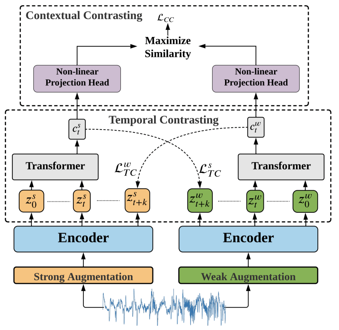
Next, the two enhanced sequences, strong and weak, are input into a convolutional temporal network to obtain the representation of each sequence at each moment. Two comparative learning methods, Temporal Contrasting and Contextual Contrasting, are used in this paper.
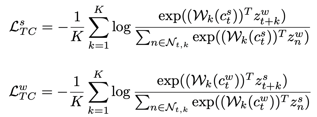
Temporal Contrasting refers to using the context of one view to predict the representation of another view in the future. The goal is to make the representation closer to the real representation corresponding to another view. Here, Transformer is used as the main model for timing prediction. The formula is as follows, where c represents the Transformer output of the strong view, Wk is a mapping function used to map c to the prediction of the future, and z is the representation of the future moment of the weak view:
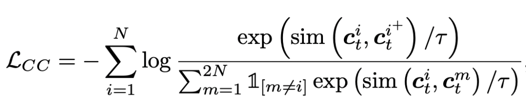
Contextual Contrasting is the comparative learning of the whole sequence, which shortens the distance between two views generated by the same sequence, and makes the distance of views generated by different sequences farther. The formula is as follows, which is similar to the method of image contrast learning:
1.2 Using Unsupervised Representation Learning
TS2Vec: Towards Universal Representation of Time Series(AAAI’22)
The core idea of TS2Vec is also unsupervised representation learning, which constructs positive sample pairs through data enhancement, and makes the distance between positive sample pairs and negative samples farther through the optimization goal of contrastive learning. The core points of this paper are mainly in two aspects. The first is the construction of positive sample pairs for the characteristics of time series and the design of the optimization goal of contrastive learning. The second is the hierarchical contrastive learning combined with the characteristics of time series.
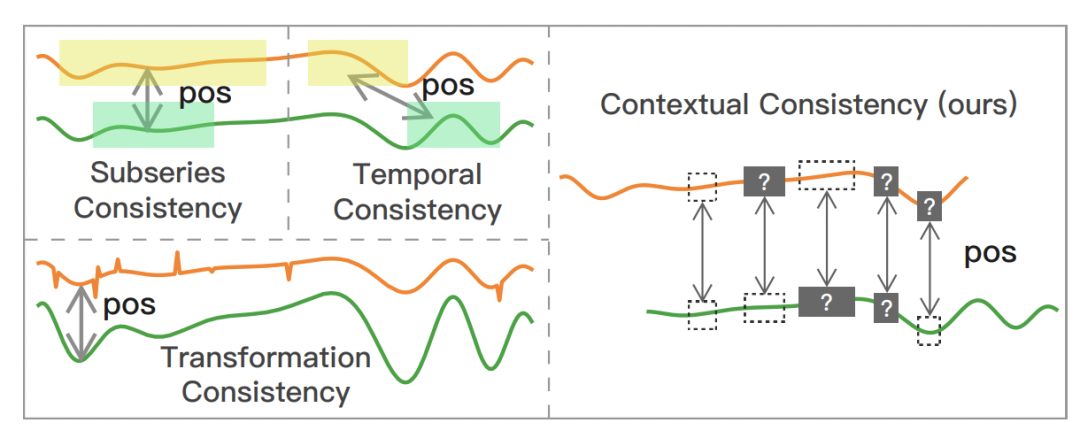
For the positive sample pair construction method, this paper proposes a positive sample pair construction method suitable for time series: Contextual Consistency. The core idea of Contextual Consistency is that the time series of two different enhanced views are closer to each other at the same time step. In this paper, two methods for constructing Contextual Consistency positive sample pairs are proposed. The first is Timestamp Masking. After full connection, the vector representation of some time steps is randomly masked, and then the representation of each time step is extracted through CNN. The second is Random Cropping, which selects two subsequences with common parts as positive sample pairs. These two methods are to make the vector representation of the same time step closer, as shown in the figure above.
Another core point of TS2Vec is hierarchical contrastive learning. An important difference between time series and images and natural language is that time series with different granularities can be obtained through aggregation at different frequencies. For example, for day-grained time series, week-grained time series can be obtained by aggregation by week, and month-grained series can be obtained by month-grained time series. In order to integrate the hierarchy of time series into contrastive learning, TS2Vec proposes hierarchical contrastive learning, and the algorithm flow is as follows.
For two time series that are mutually positive sample pairs, CNN generates a vector representation of each time step at first, and then uses maxpooling to aggregate in the time dimension. The aggregation window used in this paper is 2. After each aggregation, the distance of the aggregation vector corresponding to the time step is calculated, so that the distance of the same time step is close. The aggregation granularity keeps getting coarser, and finally aggregates into the entire time series granularity, gradually realizing instance-level representation learning.
1.3 Multivariate Time Series Representation
A transformer-based framework for multivariate time series representation learning(KDD’22)
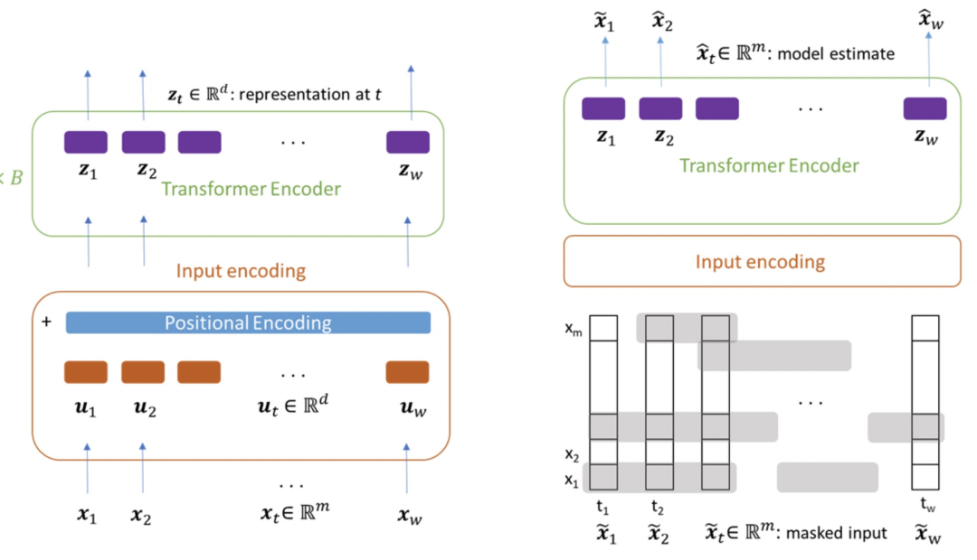
This article draws on the idea of the pre-trained language model Transformer, hoping to learn a good multivariate time series representation through an unsupervised method on the multivariate time series and with the help of the Transformer model structure. This paper focuses on unsupervised pre-training tasks designed for multivariate time series. On the right side of the figure below, for the input multivariate time series, a certain proportion of subsequences (not too short) will be masked, and each variable will be masked separately, rather than all variables in the same period of time will be masked. The optimization goal of pre-training is to restore the entire multivariate time series. In this way, when the model predicts the masked part, it can not only consider the previous and subsequent sequences, but also consider the sequence that has not been masked in the same time period.
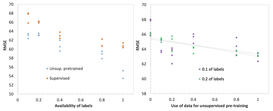
The figure below shows the improvement of the unsupervised pre-training time series model on the time series forecasting task. The figure on the left shows the comparison of the RMSE effect of whether to use unsupervised pre-training under different amounts of label data. It can be seen that no matter how much label data there is, adding unsupervised pre-training can improve the prediction effect. The figure on the right shows that the larger the amount of unsupervised pre-training data used, the better the fitting effect of the final time series forecast.
1.4 Sampling in the Timing Domain
The method proposed in this article is different from the previous article in the selection of positive and negative samples and the design of the loss function. The first is the selection of positive and negative samples. For a time series centered at time t, a Gaussian distribution is used to delineate the sampling range of its positive samples. The Gaussian distribution is centered at t, and another parameter is the extent of the time window. For the selection of the time window range, the ADF test method is used in this paper to select the optimal window span. If the time window range is too long, the sampled positive sample may not be correlated with the original sample; if the time window is too small, the sampled positive sample and the original sample may overlap too much. The ADF test can detect the time series in the stable time window, so as to select the most suitable sampling range.
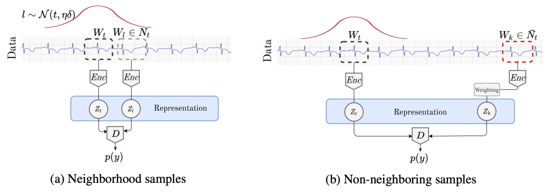
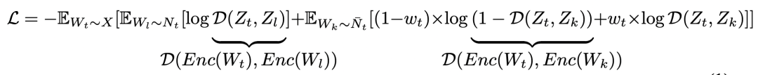
In terms of loss function, the paper mainly solves the problem of false negative samples. If all the samples outside the window selected above are regarded as negative samples, it is very likely that a pseudo-negative sample will appear, that is, it is originally related to the original sample, but it is mistaken for a negative sample because it is far away from the original sample. . For example, the time series is based on a yearly period, and the time window is selected as one month. The series of the same period last year may be considered as negative samples. This affects model training and makes it difficult for the model to converge. In order to solve this problem, this paper does not regard samples outside the window as negative samples, but as samples without labels. In the loss function, a weight is set for each sample, which represents the probability that the sample is a positive sample. This method is also known as Positive-Unlabeled (PU) learning. The final loss function can be expressed as follows:
1.5 Multivariate time series
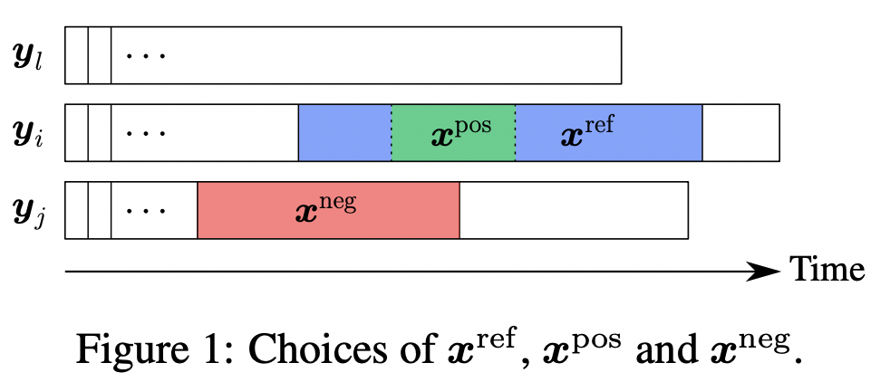
The idea of the time series representation learning method in this paper comes from the classic word vector model CBOW. The assumption in CBOW is that the contextual representation of a word should be relatively close to the representation of that word, and relatively far away from other randomly sampled word representations. This article applies this idea to time series representation learning. First, it is necessary to construct the context (context) and random negative samples in CBOW. The construction method is shown in the figure below. First select a time series xref, and a subsequence xpos in xref. , xref can be regarded as the context of xpos. At the same time, randomly sample multiple negative samples xneg from other time series, or other time segments of the current time series. In this way, a loss function similar to CBOW can be constructed, so that xref and xpos are close, while xref and other negative samples xneg are far away.
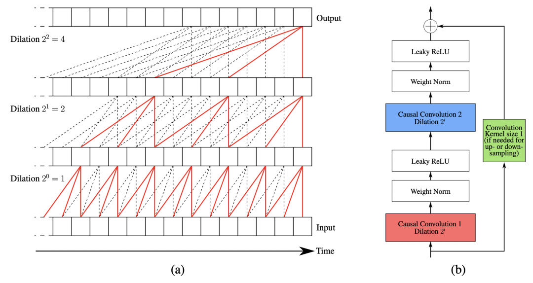
In terms of model structure, this article adopts the structure of multi-layer atrous convolution. This part of the model structure has been introduced in detail in the previous article. Interested students can refer to: 12 top conference papers, deep learning time series prediction classic scheme summary.
2. Unsupervised pre-training
Self-Supervised Contrastive Pre-Training For Time Series via Time-Frequency Consistency
先验性假设,时频一致性
The core of unsupervised pre-training is to introduce the prior into the model to learn the parameters of strong generalization. The prior introduced in this paper is that the representation of the same time series in the frequency domain and the representation in the time domain should be similar. With this as the goal, use the comparison Learn to pre-train.
2.1 Motivation
Unsupervised pre-training is used more and more in time series, but unlike NLP, CV and other fields, pre-training in time series does not have a particularly suitable prior assumption that is consistent on all data. For example, in NLP, an a priori assumption is that texts in any field or language follow the same grammatical rules. But in time series, the frequency, periodicity, and stationarity of different data sets are very different. In the previous pre-training method, some data sets are now pretrained and then finetune in the target data set. If the time series related features of the pre-trained data set and the finetune data set are very different, there will be a problem of poor migration effect.
In order to solve this problem, this paper finds a law that exists in any time series data set, that is, the frequency domain representation and time domain representation of a time series should be similar. In time series, time domain and frequency domain are two representations of the same time series, so if there is a hidden space shared by time domain and frequency domain, the representations of the two should be the same, and should be in any time series data There are the same rules.
Based on the above considerations, this paper proposes the core architecture of Time-Frequency Consistency (TF-C), which is based on comparative learning, so that the sequence representations in the time domain and frequency domain are as close as possible.
2.2 Basic Model Architecture
Based on the above ideas, the overall model structure constructed in this paper is shown in the figure below. First, a variety of time series data enhancement methods are used to generate different enhanced versions of each time series. Then input the time series into Time Encoder and Frequency Encoder to obtain the representation of time series in time domain and frequency domain respectively. Loss functions include time-domain contrastive learning loss, frequency-domain contrastive learning loss, and tabular alignment loss in time-domain and frequency-domain.
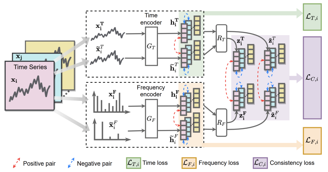
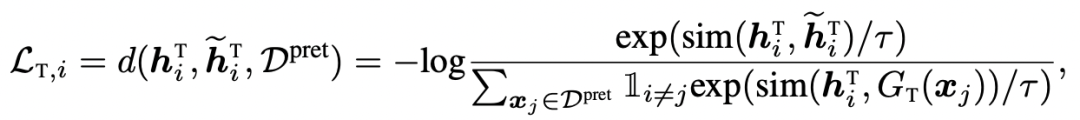
In the time domain, the data enhancement methods used include jittering, scaling, time-shifts, neighborhood segments and other classic operations in time series comparative learning (for time series data enhancement, a separate article will be published later). After Time Encoder, let a time series be similar to its enhanced result, and far away from other time series:
In the frequency domain, this paper is the first study on how to perform time series data augmentation in the frequency domain. In this paper, data enhancement in the frequency domain is achieved by erasing randomly or adding frequency components. At the same time, in order to avoid large changes in the noise of the original sequence due to the detour in the frequency domain, resulting in the dissimilarity between the enhanced sequence and the original sequence, the added and deleted components and the addition and deletion range are limited. For the delete operation, no more than E frequencies will be randomly selected for deletion; for the increase operation, those frequencies whose amplitude is less than a certain threshold will be selected and their amplitude will be increased. After obtaining the result of frequency domain data enhancement, use the Frequency Encoder to obtain the frequency domain representation, and use the comparative learning similar to the time domain for learning.
2.3 Time domain and frequency domain consistency
The above-mentioned basic model structure only uses comparative learning in the time domain and frequency domain to shorten the representation, and has not yet introduced the alignment of the time domain and frequency domain representations. In order to achieve the consistency of time domain and frequency domain, this paper designs a consistency loss to narrow the representation of the same sample in time domain and frequency domain.
The specific loss function is as follows, which mainly draws on the idea of triplet loss. Among them, STF is the distance generated by the same time series through the time-domain Encoder and the frequency-domain Encoder. Others with wavy lines indicate the sequence obtained by using some kind of enhanced sample of the sample. The assumption here is that the time-domain encoding and frequency-domain encoding of a sample should be closer, and farther away from the time-domain encoding or frequency-domain encoding of its enhanced samples.
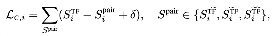
The final model is pre-trained through the combination of the above three losses.