This series of blog posts are notes for deep learning/computer vision papers, please indicate the source for reprinting

标题：Unsupervised Representation Learning with Deep Convolutional Generative Adversarial Networks

链接：[1511.06434] Unsupervised Representation Learning with Deep Convolutional Generative Adversarial Networks (arxiv.org)

Summary

In recent years, supervised learning of convolutional networks (CNNs) has been widely used in computer vision applications. In contrast, unsupervised learning of CNNs has received less attention. In this work, we hope to bridge the gap between supervised and unsupervised learning in CNNs. We introduce a class of CNNs called deep convolutional generative adversarial networks (DCGANs), which have certain architectural constraints, and demonstrate that they are strong candidates for unsupervised learning. In training on various image datasets, we show convincing evidence that our deep convolutional adversarial pairs learn a hierarchy of representations from object parts to scenes in both the generator and the discriminator. Furthermore, we use the learned features for new tasks - demonstrating their applicability as general image representations.

1 Introduction

Learning reusable feature representations from large unlabeled datasets has been an area of active research. In the context of computer vision, one can leverage virtually unlimited amounts of unlabeled images and videos to learn good intermediate representations, which can then be used for various supervised learning tasks such as image classification. We propose that one way to build good image representations is by training generative adversarial networks (GANs) (Goodfellow et al., 2014), and then reusing parts of the generator and discriminator networks as feature extractors for supervised tasks. GANs offer an attractive alternative to maximum likelihood techniques. One could also argue that their learning procedure, together with a cost function without heuristics such as pixel-independent mean square error, is attractive for representation learning. GANs are notoriously unstable, often resulting in nonsensical output from the generator. Published research is very limited in trying to understand and visualize what GANs have learned, and the intermediate representations of multi-layer GANs.

In this paper, we make the following contributions:

We propose and evaluate a set of constraints on the architectural topology of convolutional GANs that make them robust to training in most settings. We name this class of architectures Deep Convolutional Generative Adversarial Networks (DCGANs).
We use a trained discriminator for image classification tasks and demonstrate competitive performance with other unsupervised algorithms.
We visualize the filters learned by GANs and empirically show that specific filters have learned to draw specific objects.
We show that generators have interesting vector arithmetic properties that allow easy manipulation of many semantic qualities of generated samples.

2 related work

2.1 Learning representations from unlabeled data

Unsupervised representation learning is a fairly well-studied problem in general computer vision research, also in the context of images. The classic approach to unsupervised representation learning is to cluster the data (e.g. using K-means) and exploit these clusters to improve classification scores. In the context of images, image patches can be clustered hierarchically (Coates & Ng, 2012) to learn powerful image representations. Another popular approach is to train an autoencoder (convolutional, stacking (Vincent et al., 2010), what and where components of the separated code (Zhao et al., 2015), ladder structure (Rasmus et al., 2015)), where the The image is encoded into a compact code, and the code is decoded to reconstruct the image as accurately as possible. These methods have also been shown to learn good feature representations from image pixels. Deep Belief Networks (Lee et al., 2009) have also been shown to perform well at learning hierarchical representations.

2.2 Generating natural images

Generative image models have been studied intensively and fall into two categories: parametric and nonparametric. Nonparametric models typically match from databases of existing images, often patches of matched images, and have been used for texture synthesis (Efros et al., 1999), super-resolution (Freeman et al., 2002), and image inpainting ( Hays & Efros, 2007). Parametric models for generating images have been extensively explored (e.g. on MNIST digits or for texture synthesis (Portilla & Simoncelli, 2000)). However, generating real-world natural images has not had much success until recently. Variational sampling methods (Kingma & Welling, 2013) for generating images have had some success, but samples often suffer from blurring. Another approach uses an iterative forward diffusion process (Sohl-Dickstein et al., 2015) to generate images. Images generated by generative adversarial networks (Goodfellow et al., 2014) suffer from noise and incomprehension. A Laplacian Pyramid extension of this approach (Denton et al., 2015) shows higher quality images, but they still suffer from objects looking wobbly due to noise introduced when linking multiple models. Recurrent network approaches (Gregor et al., 2015) and deconvolutional network approaches (Dosovitskiy et al., 2014) have also recently shown some success in generating natural images. However, they did not utilize generators for supervised tasks.

2.3 Visualizing the internal structure of CNNs

A persistent criticism of using neural networks is that they are black-box approaches, with little understanding of what the network is doing in the form of a simple, human-digestible algorithm. In the context of CNNs, Zeiler et al. (Zeiler & Fergus, 2014) show that by using deconvolution and filtering with maximal activations, it is possible to find the approximate usage of each convolutional filter in the network. Likewise, gradient descent on the input allows us to examine ideal images that activate some subset of filters (Mordvintsev et al.).

3 Method and model architecture

Historical attempts to extend GANs to simulate images using CNNs have been unsuccessful. This prompted the authors of LAPGAN (Denton et al., 2015) to develop an alternative method that iteratively upscales low-resolution generated images that can be modeled more reliably. We also ran into difficulties trying to scale GANs with CNN architectures commonly used in the supervised literature. However, after extensive model exploration, we identify a family of architectures that are robust to training on a range of datasets and allow training higher resolution and deeper generative models.

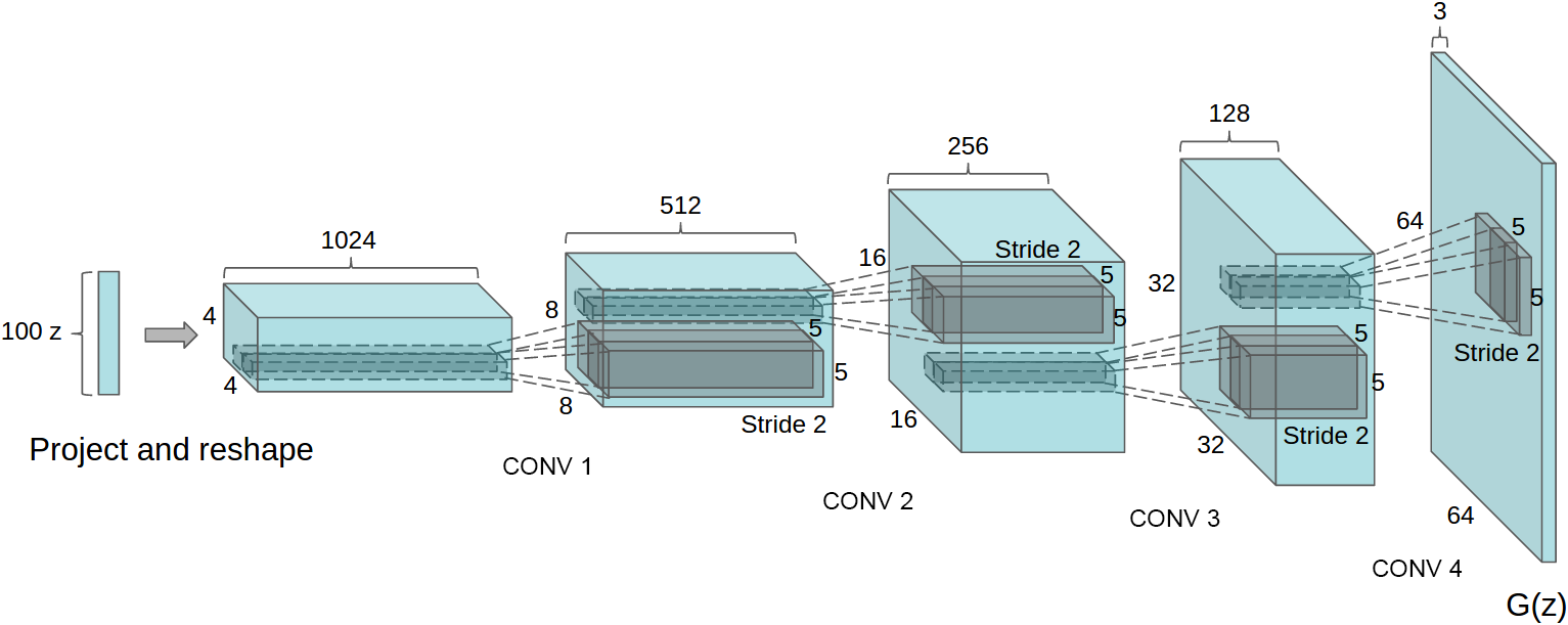
At the core of our approach is the adoption and modification of three recent changes to CNN architectures. The first is a fully convolutional network (Springenberg et al., 2014), which replaces deterministic spatial pooling functions (such as max pooling) with strided convolutions, enabling the network to learn its own spatial downsampling. We use this approach in the generator, which learns its own spatial upsampling, and the discriminator. The second is the tendency to eliminate fully connected layers on top of convolutional features. The strongest example of this is global average pooling, which has been used in state-of-the-art image classification models (Mordvintsev et al.). We find that global average pooling increases the stability of the model but reduces the convergence rate. Directly connecting the highest convolutional features to the input and output of the generator and discriminator works well. The first layer of a GAN, which takes a uniform noise distribution Z as input, can be called fully connected because it is just a matrix multiplication, but the result is reshaped into a 4-dimensional tensor and used as the start of a convolutional stack. For the discriminator, the final convolutional layer is flattened and fed into a single sigmoid output. See Figure 1 for a visualization of an example model architecture.

Figure 1: DCGAN generator for LSUN scene modeling. A 100-dimensional uniform distribution Z is mapped to a convolutional representation of a small spatial extent with many feature maps. Then, convolutions of four fractional strides (in some recent papers, these are erroneously called deconvolutions) convert this high-level representation into a 64×64 pixel image. It is worth noting that no fully connected or pooling layers are used.

The third is batch regularization (Ioffe & Szegedy, 2015), which stabilizes learning by normalizing the input to each unit to have zero mean and unit variance. This helps with training issues due to poor initialization and helps gradient flow in deeper models. This is crucial for getting the deep generator to start learning, preventing the generator from collapsing all the samples to a single point, a common failure mode observed in GANs. However, directly applying batchnorm to all layers leads to sample oscillation and model instability. This is avoided by not applying batchnorm on the output layer of the generator and the input layer of the discriminator. The ReLU activation function (Nair & Hinton, 2010) is used in the generator, except that the output layer uses the Tanh function. We observe that using bounded activations allows the model to learn more quickly to saturate and cover the color space of the training distribution. Within the discriminator, we find that leaky corrected activations (Maas et al., 2013) (Xu et al., 2015) work well, especially for high-resolution modeling. This is in contrast to the original GAN paper, which used maxout activations (Goodfellow et al., 2013).

Architectural guidelines for stable deep convolutional GANs:

Replace any pooling layers with strided convolutions (discriminator) and fractional strided convolutions (generator).

Batch normalization (batchnorm) is used in both the generator and the discriminator.

For a deeper architecture, fully connected hidden layers are removed.

In the generator, all layers except the output layer use the ReLU activation function, which uses Tanh for the output layer.

All layers in the discriminator use the LeakyReLU activation function.

4 Details of Adversarial Training

We trained DCGANs on three datasets, Large-scale Scene Understanding (LSUN) (Yu et al., 2015), Imagenet-1k, and a newly assembled face dataset. The usage details of these datasets are given below. Apart from scaling the training images to the range [-1, 1] of the tanh activation function, no preprocessing was done on the training images. All models are trained using mini-batch stochastic gradient descent (SGD), with a mini-batch size of 128. All weights were initialized from a zero-centered normal distribution with a standard deviation of 0.02. In LeakyReLU, the leaky slope is set to 0.2 for all models. While previous GAN work has used momentum to speed up training, we use the Adam optimizer (Kingma & Ba, 2014) and tune the hyperparameters. We found the suggested learning rate of 0.001 to be too high and used 0.0002 instead. Furthermore, we found that keeping the momentum term β1 at the suggested value of 0.9 leads to choppy and unstable training, while reducing it to 0.5 helps to stabilize training.

4.1 LSUN

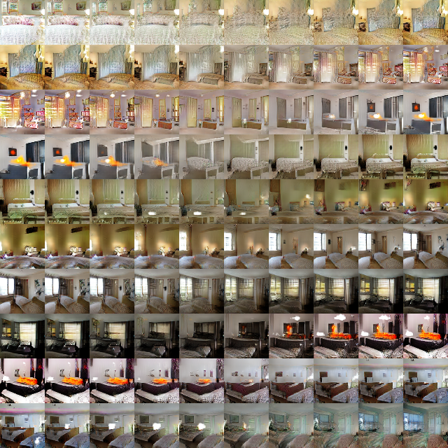
As the visual quality of samples from generative image models has improved, overfitting and memory issues of training samples have attracted attention. To show how our model scales with more data and higher-resolution generation, we train on the LSUN bedroom dataset, which contains just over 3 million training examples. Recent analyzes have shown a direct correlation between the speed at which a model learns and its generalization performance (Hardt et al., 2015). We show samples from one training epoch (Fig. 2), mimicking online learning, and samples after convergence (Fig. 3), as an opportunity to demonstrate that our model is not simply overfitting/memorizing training samples to produce high quality of samples. No data augmentation is applied on the image.

Figure 2: Bedrooms generated after one training run through the dataset. Theoretically, the model could learn to memorize the training samples, but since we train with small learning rates and mini-batch SGD, this is experimentally unlikely. We are not aware of any previous empirical evidence of memory effects using SGD and small learning rates.

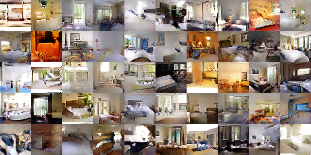
Figure 3: Bedrooms generated after training five times. There appears to be visual evidence of underfitting through repeated noise textures (such as the floor of some beds) in multiple samples.

4.1.1 Deduplication

To further reduce the possibility of the generator memorizing the input samples (Fig. 2), we perform a simple image deduplication process. We fit a 3072-128-3072 denoising dropout regularized ReLU autoencoder on a 32 × 32 downsampled center crop of the training samples. The resulting code layer activations are then binarized by thresholding the ReLU activations, which has been shown to be an effective information-preserving technique (Srivastava et al., 2014) and provides a convenient form of semantic hashing that allows Linear time deduplication. Visual inspection of hash collisions shows high accuracy, with an estimated false positive rate of less than 1/100. Furthermore, this technique detected and removed approximately 275,000 near-duplicates, indicating a high recall rate.

4.2 Face

We crawled images containing faces from random web image queries. The names of these people are taken from dbpedia, and the criterion is that they were born in the modern era. This dataset has 3 million images from 10,000 individuals. We ran an OpenCV face detector on these images, retaining a high enough resolution to give us around 350,000 face boxes. We use these face boxes for training. No data augmentation is applied on the image.

4.3 IMAGENET-1K

We use Imagenet-1k (Deng et al., 2009) as the natural image source for unsupervised training. We train on the smallest size on a 32 × 32 center crop. No data augmentation is applied on the image.

5 Empirical verification of DCGANs

5.1 Classification of CIFAR-10 using GAN as feature extractor

A common technique for evaluating the quality of an unsupervised representation learning algorithm is to apply it as a feature extractor to a supervised dataset and evaluate the performance of a linear model based on these features.

On the CIFAR-10 dataset, a single-layer feature extraction pipeline using K-means as a feature learning algorithm has demonstrated very strong baseline performance. When using a large number of feature maps (4800), this technique achieves 80.6% accuracy. An unsupervised multi-layer extension of the underlying algorithm achieved an accuracy of 82.0% (Coates & Ng, 2011). To evaluate the quality of representations learned by DCGANs for supervised tasks, we train on Imagenet-1k, then use the convolutional features of all layers of the discriminator to max-pool the representations of each layer, resulting in a 4 × 4 space grid. These features are then flattened and concatenated to form a 28672-dimensional vector, after which a regularized linear L2-SVM classifier is trained on it. This achieves an accuracy of 82.8%, surpassing all K-means based methods. It is worth noting that the discriminator has fewer feature maps (512 at the highest layer) compared to K-means based techniques, but due to the multiple layers of 4 × 4 spatial locations, the result is larger in total feature vector size has increased. The performance of DCGANs is still lower than that of example CNNs (Dosovitskiy et al., 2015), which is an unsupervised way to train normal discriminative CNNs to distinguish specifically selected, heavily enhanced, examples from the source dataset. sample. Further improvements can be made by fine-tuning the representation of the discriminator, but we leave this as future work. Furthermore, since our DCGAN has never been trained on CIFAR-10, this experiment also demonstrates the domain robustness of the learned features.

Table 1: Classification results on CIFAR-10 using our pretrained model. Our DCGAN is not pre-trained on CIFAR-10, but on Imagenet-1k, and then uses these features to classify CIFAR-10 images.

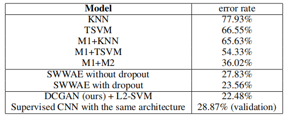
5.2 Classifying SVHN digits using GAN as feature extractor

On the Street View House Numbers dataset (SVHN) (Netzer et al., 2011), we use the features of the discriminator of DCGAN for supervision purposes when labeled data is scarce. Following similar dataset preparation rules as in the CIFAR-10 experiments, we separate a validation set of 10,000 samples from the non-extra set and use it for all hyperparameter and model selection. Randomly select 1000 uniformly distributed category training samples, and train a regularized linear L2-SVM classifier on the same feature extraction pipeline used on CIFAR-10. This achieves a test error of 22.48%, improving on another modification of CNNs aimed at exploiting unlabeled data (Zhao et al., 2015). Furthermore, we verify that the CNN architecture used in DCGAN is not the main contributor to model performance by training a purely supervised CNN on the same data and using the same architecture by performing random search optimization on 64 hyperparameter trials. This model (Bergstra & Bengio, 2012). It achieves a higher validation error of 28.87%.

6 Studying and Visualizing the Internal Structure of a Network

We study already trained generators and discriminators in various ways. We did not perform any kind of nearest neighbor search on the training set. Pixel or nearest neighbors in feature space are easily fooled by small image transformations (Theis et al., 2015). We also did not use the log-likelihood metric to evaluate models quantitatively, as it is a poor evaluation metric (Theis et al., 2015).

Table 2: Classifying SVHN with 1000 labels

6.1 Walking in the latent space

The first experiment we performed was to understand the structure of the latent space. Walking the learned manifold can often tell us about signs of memorization (if there are sudden transitions), and how hierarchically the space collapses. If walking in this latent space results in semantic changes to image generation (such as the addition and removal of objects), we can infer that the model has learned relevant and interesting representations. The results are shown in Figure 4.

Figure 4: Top rows: Interpolation between 9 random points in Z shows that the learned space has smooth transitions, and each image in the space resembles a bedroom. On row 6, you can see a windowless room slowly turning into a room with huge windows. On line 10, you can see what appears to be a TV slowly turning into a window.

6.2 Visualizing Discriminator Features

Previous work has demonstrated that supervised training of CNNs on large image datasets can yield very powerful learned features (Zeiler & Fergus, 2014). Furthermore, supervised CNNs for scene classification can learn object detectors (Oquab et al., 2014). We demonstrate that a DCGAN trained unsupervised on a large image dataset can also learn a range of interesting features. Using guided backpropagation as proposed in (Springenberg et al., 2014), we show in Figure 5 the activation of the features learned by the discriminator on typical parts of a bedroom such as a bed and windows. For comparison, we present in the same figure a baseline of randomly initialized features that do not activate anything semantically relevant or interesting.

Figure 5: Shown on the right is a guided backpropagation visualization of the maximum axial response of the first 6 learned convolutional features in the last convolutional layer of the discriminator. Note that a considerable number of features respond to beds - this is the central object in the LSUN bedroom dataset. On the left is a baseline with a random filter. Compared to the previous responses, here there is little discrimination and random structure.

6.3 Manipulating generator representations

6.3.1 Forgot to draw some objects

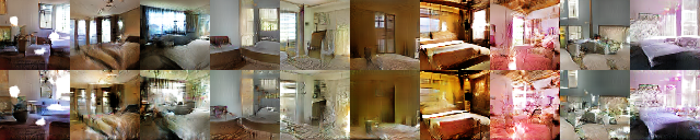
In addition to the representations learned by the discriminator, there is also the problem of representations learned by the generator. The quality of the samples indicates that the generator learned object-specific representations of major scene components such as beds, windows, lights, doors, and miscellaneous furniture. To explore the form of these representations, we conducted an experiment trying to remove windows from the generator entirely.

On 150 samples, 52 window bounding boxes are drawn by hand. On the second highest convolutional layer feature, a logistic regression was fitted to predict whether the feature activation is within a window by using the criteria that the activation within the drawn bounding box is positive and a random sample from the same image is negative. on (or not on). Using this simple model, all feature maps with weights greater than zero (200 in total) are removed from all spatial locations. Then, random new samples with and without feature map removal were generated.

The generated images with and without window loss are shown in Fig. 6. Interestingly, the network mostly forgot to draw windows in bedrooms, replacing them with other objects.

Figure 6: Top row: Unmodified samples from the model. Bottom row: The same sample generated after removing the "windows" filter. Some windows were removed, others were transformed into visually similar objects such as doors and mirrors. Despite the drop in visual quality, the overall scene composition remains similar, implying that the generator does a good job of decoupling the scene representation from the object representation. Extended experiments can be performed to remove other objects from the image and modify the objects drawn by the generator.

6.3.2 Vector Arithmetic on Face Samples

In the context of evaluating learned word representations, Mikolov et al. (2013) show that simple arithmetic operations reveal rich linear structures in the representation space. A classic example shows that the result of vector("King") - vector("Man") + vector("Woman") is a vector that is the nearest neighbor to the Queen vector. We investigate whether a similar structure exists in the Z representation of our generator. We perform similar arithmetic operations on the Z-vectors of a typical set of samples of visual concepts. Experiments based on only a single sample of each concept were unstable, but averaging the Z-vectors of three samples produced consistent and stable generation results that semantically followed the arithmetic. In addition to the object manipulation shown in (Fig. 7), we show that facial pose is also modeled linearly in Z space (Fig. 8).

Figure 7: Vector arithmetic for visual concepts. For each column, the Z vectors of the samples are averaged. Arithmetic operations are then performed on the mean vector to create a new vector Y. The sample in the middle on the right was produced by feeding Y as input to the generator. To demonstrate the interpolation capabilities of the generator, uniform noise samples (with a scale of ±0.25) were added to Y, yielding 8 other samples. Applying arithmetic on the input space (two examples below) results in noisy overlap due to misalignment.

Figure 8: A "turn" vector is created by averaging four samples of faces looking left and right. By adding interpolation to random samples on this axis, we are able to reliably transform their poses.

These demonstrations show that interesting applications can be developed using the Z representations learned by our model. It has been previously demonstrated that conditional generative models can learn to convincingly model object properties such as scale, rotation, and position (Dosovitskiy et al., 2014). To our knowledge, this is the first demonstration in a purely unsupervised model. Further exploration and development of the vector arithmetic described above may substantially reduce the amount of data required for conditional generation to model complex image distributions.

7 Conclusions and future work

We propose a more stable architecture for training generative adversarial networks and provide evidence that adversarial networks learn good representations of images for supervised learning and generative modeling. There are also some forms of model instability - we noticed that as models trained over time, they sometimes collapsed part of the filters into a single oscillatory mode. Further work is needed to address this instability. We thought it would be interesting to extend this framework to other domains such as video (for frame prediction) and audio (pretrained features for speech synthesis). It would also be interesting to conduct further studies on the properties of the learned latent space.

thank you

In this work we have been very fortunate and grateful for all the advice and guidance we have received, especially those of Ian Goodfellow, Tobias Springenberg, Arthur Szlam and Durk Kingma. In addition, we would like to thank all colleagues at indico for their support, resources and communication, especially two other members of the indico research team, Dan Kuster and Nathan Lintz. Finally, we would like to thank Nvidia for donating the Titan-X GPUs used in this work.

references

Bergstra, James & Bengio, Yoshua. (2012). Random search for hyperparameter optimization. JMLR .
Coates, Adam & Ng, Andrew. (2011). Receptive Field Selection in Deep Networks. NIPS .
Coates, Adam & Ng, Andrew Y. (2012). Learning feature representations using k-means. In Neural Networks: Know-How of the Trade (pp. 561–580). Springer.
Deng, Jia, Dong, Wei, Socher, Richard, Li, Li-Jia, Li, Kai, & Fei-Fei, Li. (2009). ImageNet: A Large-Scale Hierarchical Image Database. In Computer Vision and Pattern Recognition, 2009. IEEE Computer Society (pp. 248–255). IEEE.
Denton, Emily, Chintala, Soumith, Szlam, Arthur, & Fergus, Rob. (2015). Deep Generative Image Models Using Laplacian Pyramid Adversarial Networks. arXiv preprint arXiv:1506.05751 .
Dosovitskiy, Alexey, Springenberg, Jost Tobias, & Brox, Thomas. (2014). Chair Generation Using Convolutional Neural Networks. arXiv preprint arXiv:1411.5928 .
Dosovitskiy, Alexey et al. (2015). Discriminative Unsupervised Feature Learning with On-Sample Convolutional Neural Networks. Pattern Analysis and Machine Intelligence, IEEE Transactions on Volume 99. IEEE.
Efros, Alexei et al. (1999). Nonparametric sampling for texture synthesis. In Computer Vision, Proceedings of the Seventh IEEE International Conference , Vol. 2, pp. 1033–1038. IEEE.
Freeman, William T. et al. (2002). Example-Based Super-Resolution. Computer Graphics and Applications, IEEE , 22(2):56–65.
Goodfellow, Ian J. et al. (2013). Maxout Networks. arXiv preprint arXiv:1302.4389 .
Goodfellow, Ian J. et al. (2014). Generative Adversarial Networks. NIPS .
Gregor, Karol et al. (2015). Draw: A Recurrent Neural Network for Image Generation. arXiv preprint arXiv:1502.04623 .
Hardt, Moritz et al. (2015). Train faster, generalize better: Stability in stochastic gradient descent. arXiv preprint arXiv:1509.01240 .
Hauberg, Sren et al. (2015). Dreaming More Data: Class-Dependent Differential Manifold Distributions for Learning Data Augmentation. arXiv preprint arXiv:1510.02795 .
Hays, James & Efros, Alexei A. (2007). Scene completion using millions of photos. ACM Transactions on Graphics (TOG) , 26(3):4.
Ioffe, Sergey & Szegedy, Christian. (2015). Batch Normalization: Accelerating Deep Network Training by Reducing Internal Covariate Shift. arXiv preprint arXiv:1502.03167 .
Kingma, Diederik P. & Ba, Jimmy Lei. (2014). Adam: A Stochastic Optimization Method. arXiv preprint arXiv:1412.6980 .
Kingma, Diederik P. & Welling, Max. (2013). Autoencoding Variational Bayesian. arXiv preprint arXiv:1312.6114 .
Lee, Honglak et al. (2009). Convolutional Deep Belief Networks for Scalable Unsupervised Learning of Hierarchical Representations. In Proceedings of the 26th International Conference on Machine Learning , pp. 609–616. ACM.
Loosli, Gaëlle et al. (2007). Training Invariant Support Vector Machines Using Selective Sampling. In Large-Scale Nuclear Machines , pp. 301–320. MIT Press, Cambridge, MA.
Maas, Andrew L. et al. (2013). Rectifier nonlinearity improves neural network acoustic models. ICML Conference Proceedings , Vol. 30.
Mikolov, Tomas et al. (2013). Distributional representations of words and phrases and their compositionality. Advances in Neural Information Processing Systems , pp. 3111–3119.
Mordvintsev, Alexander et al. Introspectionism: A Deeper Exploration of Neural Networks. Google Research Blog. [online]. Accessed: 17 June 2015.
Nair, Vinod & Hinton, Geoffrey E. (2010). Rectified linear units improve restricted Boltzmann machines. Proceedings of the 27th Annual International Conference on Machine Learning (ICML-10) , pp. 807–814.
Netzer, Yuval et al. (2011). Reading digits in natural images using unsupervised feature learning. In NIPS Workshop on Deep Learning and Unsupervised Feature Learning , Volume 2011, Page 5. Granada, Spain.
Oquab, M. et al. (2014). Learning and Transferring Mid-Level Image Representations Using Convolutional Neural Networks. at CVPR .
Portilla, Javier & Simoncelli, Eero P. (2000). Parametric texture models based on joint statistics of complex wavelet coefficients. International Journal of Computer Vision , 40(1): 49–70.
Rasmus, Antti et al. (2015). Semi-supervised learning with gradient-climbing ladder networks. arXiv preprint arXiv:1507.02672 .
Sohl-Dickstein, Jascha et al. (2015). Deep Unsupervised Learning Using Nonequilibrium Thermodynamics. arXiv preprint arXiv:1503.03585 .
Springenberg, Jost Tobias et al. (2014). In Pursuit of Simplicity: Fully Convolutional Networks. arXiv preprint arXiv:1412.6806 .
Srivastava, Rupesh Kumar et al. (2014). Understanding Local Competitive Networks. arXiv preprint arXiv:1410.1165 .
Theis, L. et al. (2015). Notes on Generative Model Evaluation. arXiv:1511.01844 .
Vincent, Pascal et al. (2010). Stacked Denoising Autoencoders: Learning Useful Representations in Deep Networks with Local Denoising Criteria. Journal of Machine Learning Research , 11:3371–3408.
Xu, Bing et al. (2015). Empirically evaluating rectified activations in convolutional networks. arXiv preprint arXiv:1505.00853 .
Yu, Fisher et al. (2015). Building Large-Scale Image Datasets Using Deep Learning with People in the Loop. arXiv preprint arXiv:1506.03365 .
Zeiler, Matthew D & Fergus, Rob. (2014). Visualizing and Understanding Convolutional Networks. In Computer Vision – ECCV 2014 , pp. 818–833. Springer.
Zhao, Junbo et al. (2015). Stacking what-where autoencoders. arXiv preprint arXiv:1506.02351 .

REFERENCES

Bergstra, James & Bengio, Yoshua. (2012). Random search for hyper-parameter optimization. JMLR.
Coates, Adam & Ng, Andrew. (2011). Selecting receptive fields in deep networks. NIPS.
Coates, Adam & Ng, Andrew Y. (2012). Learning feature representations with k-means. In Neural Networks: Tricks of the Trade (pp. 561–580). Springer.
Deng, Jia, Dong, Wei, Socher, Richard, Li, Li-Jia, Li, Kai, & Fei-Fei, Li. (2009). Imagenet: A large-scale hierarchical image database. In Computer Vision and Pattern Recognition , 2009. CVPR 2009. IEEE Conference on (pp. 248–255). IEEE.
Denton, Emily, Chintala, Soumith, Szlam, Arthur, & Fergus, Rob. (2015). Deep generative image models using a laplacian pyramid of adversarial networks. arXiv preprint arXiv:1506.05751.
Dosovitskiy, Alexey, Springenberg, Jost Tobias, & Brox, Thomas. (2014). Learning to generate chairs with convolutional neural networks. arXiv preprint arXiv:1411.5928.
Dosovitskiy, Alexey et al. (2015). Discriminative unsupervised feature learning with exemplar convolutional neural networks. Pattern Analysis and Machine Intelligence, IEEE Transactions on, volume 99. IEEE.
Efros, Alexei et al. (1999). Texture synthesis by non-parametric sampling. In Computer Vision, The Proceedings of the Seventh IEEE International Conference on, volume 2, pp. 1033–1038. IEEE.
Freeman, William T. et al. (2002). Example-based super-resolution. Computer Graphics and Applications, IEEE, 22(2):56–65.
Goodfellow, Ian J. et al. (2013). Maxout networks. arXiv preprint arXiv:1302.4389.
Goodfellow, Ian J. et al. (2014). Generative adversarial nets. NIPS.
Gregor, Karol et al. (2015). Draw: A recurrent neural network for image generation. arXiv preprint arXiv:1502.04623.
Hardt, Moritz et al. (2015). Train faster, generalize better: Stability of stochastic gradient descent. arXiv preprint arXiv:1509.01240.
Hauberg, Sren et al. (2015). Dreaming more data: Class-dependent distributions over diffeomorphisms for learned data augmentation. arXiv preprint arXiv:1510.02795.
Hays, James & Efros, Alexei A. (2007). Scene completion using millions of photographs. ACM Transactions on Graphics (TOG), 26(3):4.
Ioffe, Sergey & Szegedy, Christian. (2015). Batch normalization: Accelerating deep network training by reducing internal covariate shift. arXiv preprint arXiv:1502.03167.
Kingma, Diederik P. & Ba, Jimmy Lei. (2014). Adam: A method for stochastic optimization. arXiv preprint arXiv:1412.6980.
Kingma, Diederik P. & Welling, Max. (2013). Auto-encoding variational bayes. arXiv preprint arXiv:1312.6114.
Lee, Honglak et al. (2009). Convolutional deep belief networks for scalable unsupervised learning of hierarchical representations. In Proceedings of the 26th Annual International Conference on Machine Learning, pp. 609–616. ACM.
Loosli, Gaëlle et al. (2007). Training invariant support vector machines using selective sampling. In Large Scale Kernel Machines, pp. 301–320. MIT Press, Cambridge, MA.
Maas, Andrew L. et al. (2013). Rectifier nonlinearities improve neural network acoustic models. Proc. ICML, volume 30.
Mikolov, Tomas et al. (2013). Distributed representations of words and phrases and their compositionality. In Advances in neural information processing systems, pp. 3111–3119.
Mordvintsev, Alexander et al. Inceptionism: Going deeper into neural networks. Google Research Blog. [Online]. Accessed: 2015-06-17.
Nair, Vinod & Hinton, Geoffrey E. (2010). Rectified linear units improve restricted boltzmann machines. Proceedings of the 27th International Conference on Machine Learning (ICML-10), pp. 807–814.
Netzer, Yuval et al. (2011). Reading digits in natural images with unsupervised feature learning. In NIPS workshop on deep learning and unsupervised feature learning, volume 2011, pp. 5. Granada, Spain.
Oquab, M. et al. (2014). Learning and transferring mid-level image representations using convolutional neural networks. In CVPR.
Portilla, Javier & Simoncelli, Eero P. (2000). A parametric texture model based on joint statistics of complex wavelet coefficients. International Journal of Computer Vision, 40(1):49–70.
Rasmus, Antti et al. (2015). Semi-supervised learning with ladder network. arXiv preprint arXiv:1507.02672.
Sohl-Dickstein, Jascha et al. (2015). Deep unsupervised learning using nonequilibrium thermodynamics. arXiv preprint arXiv:1503.03585.
Springenberg, Jost Tobias et al. (2014). Striving for simplicity: The all convolutional net. arXiv preprint arXiv:1412.6806.
Srivastava, Rupesh Kumar et al. (2014). Understanding locally competitive networks. arXiv preprint arXiv:1410.1165.
Theis, L. et al. (2015). A note on the evaluation of generative models. arXiv:1511.01844.
Vincent, Pascal et al. (2010). Stacked denoising autoencoders: Learning useful representations in a deep network with a local denoising criterion. The Journal of Machine Learning Research, 11:3371–3408.
Xu, Bing et al. (2015). Empirical evaluation of rectified activations in convolutional network. arXiv preprint arXiv:1505.00853.
Yu, Fisher et al. (2015). Construction of a large-scale image dataset using deep learning with humans in the loop. arXiv preprint arXiv:1506.03365.
Zeiler, Matthew D & Fergus, Rob. (2014). Visualizing and understanding convolutional networks. In Computer Vision–ECCV 2014, pp. 818–833. Springer.
Zhao, Junbo et al. (2015). Stacked what-where auto-encoders. arXiv preprint arXiv:1506.02351.

8 Additional material

8.1 Evaluating DCGAN's ability to capture data distributions

We propose to apply standard classification metrics on a conditional version of our model, evaluating the learned conditional distribution. We trained a DCGAN on the MNIST dataset (using 10,000 samples from it as a validation set), along with a permutation-invariant GAN baseline, and evaluated these models using nearest neighbor classifiers, comparing real data Compare to a set of generated conditional samples. We found that removing the scale and bias parameters from batch normalization leads to better results for both models. We speculate that the noise introduced by batch normalization helps generative models better explore the underlying data distribution and generate samples from it. The results are presented in Table 3, which compares our model with other techniques. The DCGAN model achieves the same level of test error as the nearest neighbor classifier fitted on the training dataset, indicating that the DCGAN model does an excellent job of modeling the conditional distribution of this dataset. At one million samples per class, the DCGAN model outperforms InfiMNIST (Loosli et al., 2007), a hand-developed data augmentation pipeline that uses translation and elastic deformation of training samples. DCGAN outperforms a probabilistic generative data augmentation technique (Hauberg et al., 2015) that uses learned per-class transformations, while being more general since it directly models the data rather than transformations of the data.

Table 3: Nearest Neighbor Classification Results

Figure 9: Side-by-side example plots (left to right) showing the MNIST dataset, baseline GAN generation, and our DCGAN generation results.

Figure 10: More generated images from our face DCGAN.

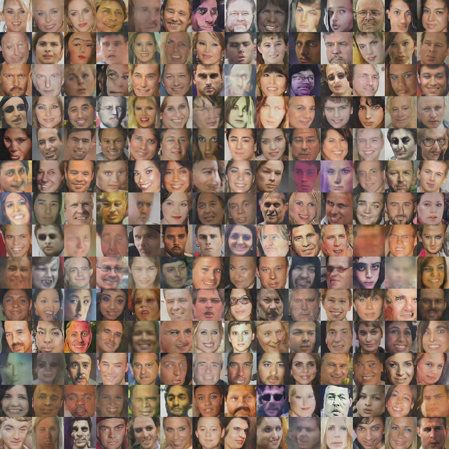
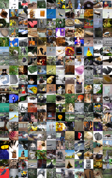
Figure 11: Generated images of a DCGAN trained on the Imagenet-1k dataset.

[Computer Vision|Generate Confrontation] Unsupervised Representation Learning with Deep Convolutional Generative Confrontation Network (DCGAN)