Python application examples (2) data visualization (1)

Data visualization refers to exploring data through visual representations. It is closely related to data analysis, which refers to using code to explore patterns and associations in data sets. Datasets can range from small lists of numbers represented by a single line of code to gigabytes of data.

Presenting data beautifully is not just about pretty pictures. By presenting data in a compelling and simple way, it makes sense to the viewer: discovering patterns and meanings in data sets that were otherwise unknown.

Fortunately, you can visualize complex data even without a supercomputer. Given Python's efficiency, it is possible to quickly explore datasets consisting of millions of data points on a laptop. Data points do not have to be numbers. Using the basics introduced in the first half of the book, non-numeric data can also be analyzed.

In many fields such as genetic research, weather research, political and economic analysis, people often use Python to complete data-intensive work. Data scientists have written an excellent set of visualization and analysis tools in Python, many of which are at your disposal. One of the most popular tools is Matplotlib, which is a mathematical plotting library that we will use to make simple charts such as line charts and scatterplots. Then, we'll generate a more interesting dataset based on the random walk concept - a graph generated from a series of random decisions.

We use the Plotly package, which generates charts that are great for displaying on digital devices. Plotly-generated charts can be automatically resized according to the size of the display device, and also have many interactive features, such as highlighting specific aspects of the data set when the user points the mouse to different parts of the chart. In this chapter, we will use Plotly to analyze the results of rolling dice.

1. Install Matplotlib

First use Matplotlib to generate a few charts, for which you need to install it using pip. pip is a module that can be used to download and install Python packages. Please execute the following command at the terminal prompt:

$ python -m pip install --user matplotlib

This command tells Python to run the module pip and add the matplotlib package to the current user's Python installation. On your system, if you run a program or start a terminal session with python3 instead of python, use a command similar to the following:

$ python3 -m pip install --user matplotlib

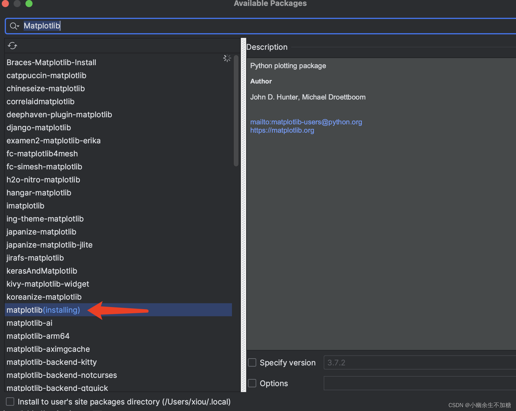
You can also search and install directly in pycharm:

2. Draw a simple line chart

Let's use Matplotlib to draw a simple line chart, and then customize it to achieve a more informative data visualization. We'll use the sequence of square numbers 1, 4, 9, 16, and 25 to make this chart. Just provide numbers like this and Matplotlib will do the rest: mpl_squares.py

  import matplotlib.pyplot as plt

  squares = [1, 4, 9, 16, 25]
❶ fig, ax = plt.subplots()
  ax.plot(squares)

  plt.show()

First import the module pyplot and assign it an alias plt to avoid repeatedly typing pyplot. (Examples online mostly do this, and here is no exception.) The module pyplot contains many functions for generating plots.

We create a list called squares where we store the data we will use to make the chart. Then, another common Matplotlib practice is adopted-calling the function subplots() (see ❶). This function draws one or more charts in one image. The variable fig represents the entire picture. The variable ax represents the individual charts in the picture, which is used in most cases.

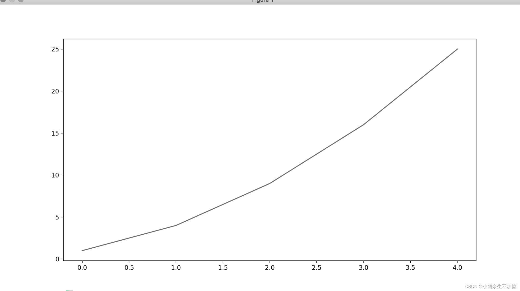
The method plot() is called next, which attempts to draw a graph in a meaningful way from the given data. The function plt.show() opens the Matplotlib viewer and displays the plotted chart, as shown in Figure 15-1. In the viewer, you can zoom and navigate the graph, and click the disk icon to save the graph.

2.1 Modify label text and line thickness

The graph shown in Figure 15-1 shows that the number is getting bigger and bigger, but the label text is too small and the lines are too thin to see clearly. Fortunately, Matplotlib lets you tweak every aspect of the visualization. Let's improve the readability of this graph with some customization, as follows: mpl_squares.py

  import matplotlib.pyplot as plt

  squares = [1, 4, 9, 16, 25]

  fig, ax = plt.subplots()
❶ ax.plot(squares, linewidth=3)

  # 设置图表标题并给坐标轴加上标签1。
❷ ax.set_title("平方数", fontsize=24)
❸ ax.set_xlabel("值", fontsize=14)
  ax.set_ylabel("值的平方", fontsize=14)

  # 设置刻度标记的大小。
❹ ax.tick_params(axis='both', labelsize=14)

  plt.show()

The parameter linewidth (see ❶) determines the thickness of the line drawn by plot(). The method set_title() (see ❷) assigns a title to the chart. In the above code, the parameter fontsize that appears multiple times specifies the size of various characters in the chart.

The methods set_xlabel() and set_ylabel() allow you to set a title for each axis (see ❸). The method tick_params() sets the style of the ticks (see ❹), where the specified arguments will affect the [inset] axis and the ticks on the [inset] axis (axes='both'), and set the font size of the tick marks to 14 ( labelsize=14).

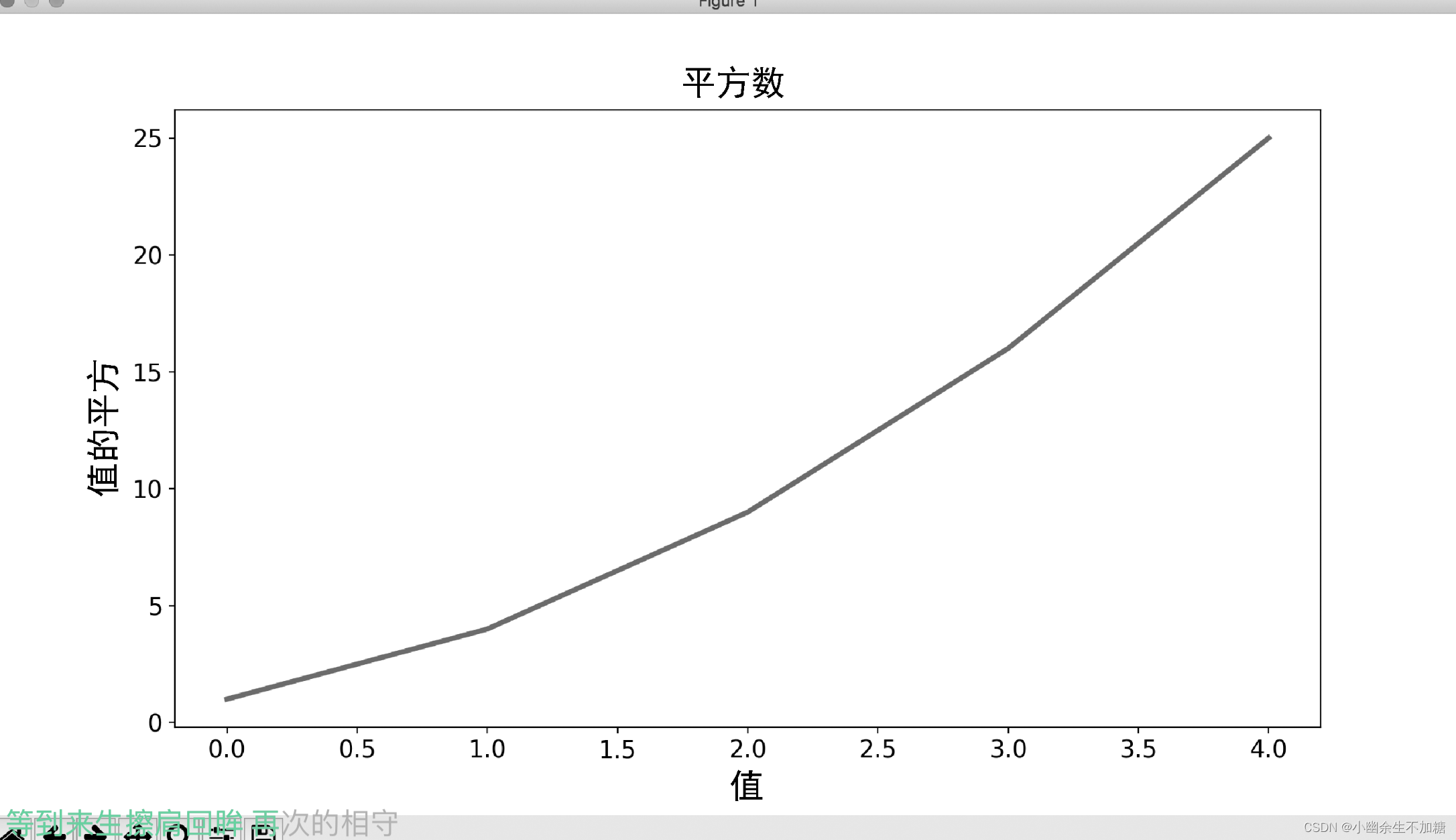
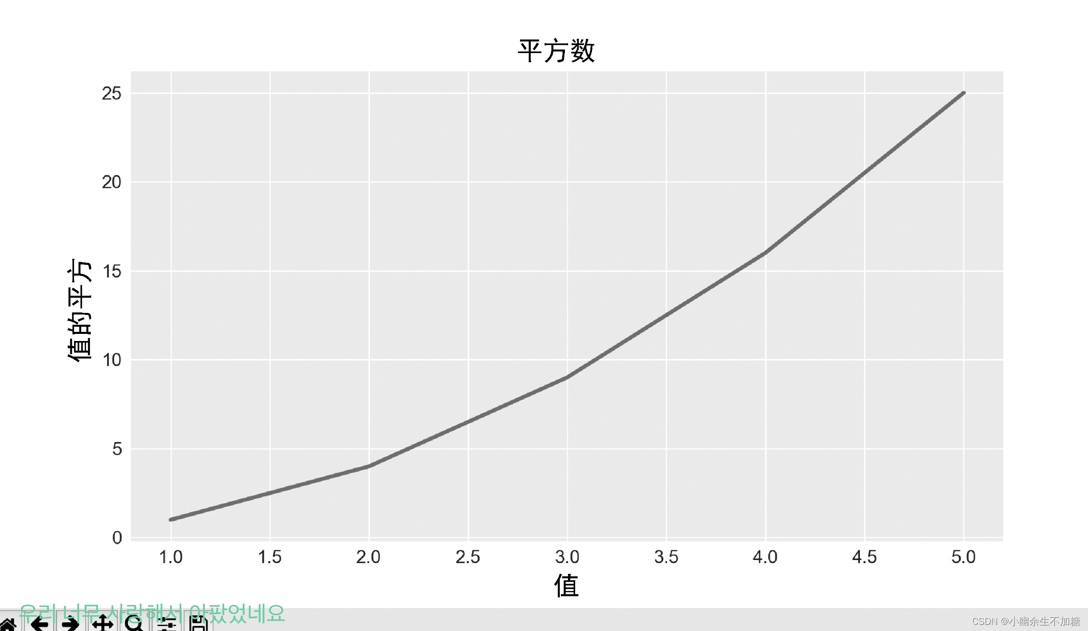
The final chart is much easier to read, as shown in Figure 15-2: the label text is larger and the lines are thicker. Often, it will be necessary to experiment with different values ​​to determine which settings produce the best graphs.

2.2 Correct graphics

Once the graph was easier to see, we discovered that the data was not plotted correctly: the endpoint of the line chart indicated that the square of 4.0 is 25! Let's fix this problem.

When you feed plot() a series of numbers, it assumes that the first data point corresponds to an [inset] value of 0, but here the first point corresponds to an [inset] value of 1. To override this default behavior, both input and output values ​​can be supplied to plot():

mpl_squares.py

import matplotlib.pyplot as plt

input_values = [1, 2, 3, 4, 5]
squares = [1, 4, 9, 16, 25]

fig, ax = plt.subplots()
ax.plot(input_values, squares, linewidth=3)

# 设置图表标题并给坐标轴加上标签。
--snip--

Now plot() will plot the data correctly, because both input and output values ​​are provided, and plot() does not have to make assumptions about how the output values ​​are generated. The final graph is correct, as shown in

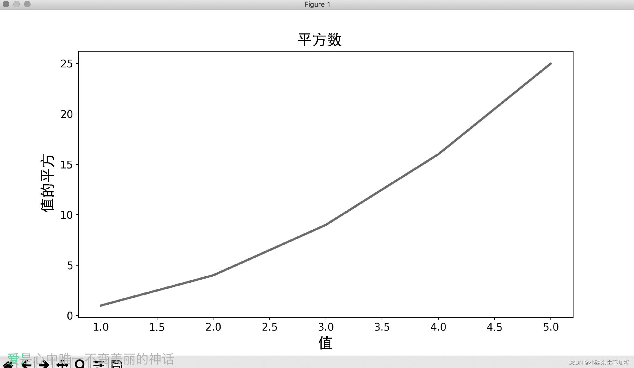
Various arguments can be specified when using plot(), and numerous functions can be used to customize the graph. These custom functions will continue to be explored later in this chapter when we deal with more interesting datasets.

2.3 Using built-in styles

Matplotlib provides a lot of well-defined styles. The background color, grid line, line thickness, font, font size, etc. settings they use are very good, so that you can generate eye-catching visualization effects without much customization. To see which styles are available on your system, execute the following command in a terminal session:

>>> import matplotlib.pyplot as plt
>>> plt.style.available
['seaborn-dark', 'seaborn-darkgrid', 'seaborn-ticks', 'fivethirtyeight',
--snip--

You can add the following line of code before the code that generates the chart: mpl_squares.py

import matplotlib.pyplot as plt

input_values = [1, 2, 3, 4, 5]
squares = [1, 4, 9, 16, 25]

plt.style.use('seaborn')
fig, ax = plt.subplots()
--snip--

The graph generated by these codes is shown in the figure. There are many built-in styles available, try them out and find what you like.

2.4 Use scatter() to draw a scatter plot and set the style

Sometimes it is useful to plot a scatterplot and style the individual data points. For example, you might want to display smaller values ​​in one color and larger values ​​in another. When plotting large datasets, it is also possible to style every point the same, and then redraw certain points with different styling options to stand out.

To plot a single point, use the method scatter(). Pass it a pair of [inset]coordinates and [inset]coordinates and it will draw a point at the specified location:

catter_squares.py

import matplotlib.pyplot as plt

plt.style.use('seaborn')
fig, ax = plt.subplots()
ax.scatter(2, 4)

plt.show()

Let's style the chart to make it more interesting. We'll add a title, label the axes, and make sure all text is big enough to read:

  import matplotlib.pyplot as plt

  plt.style.use('seaborn')
  fig, ax = plt.subplots()
❶ ax.scatter(2, 4, s=200)

  # 设置图表标题并给坐标轴加上标签。
  ax.set_title("平方数", fontsize=24)
  ax.set_xlabel("值", fontsize=14)
  ax.set_ylabel("值的平方", fontsize=14)

  # 设置刻度标记的大小。
  ax.tick_params(axis='both', which='major', labelsize=14)

  plt.show()

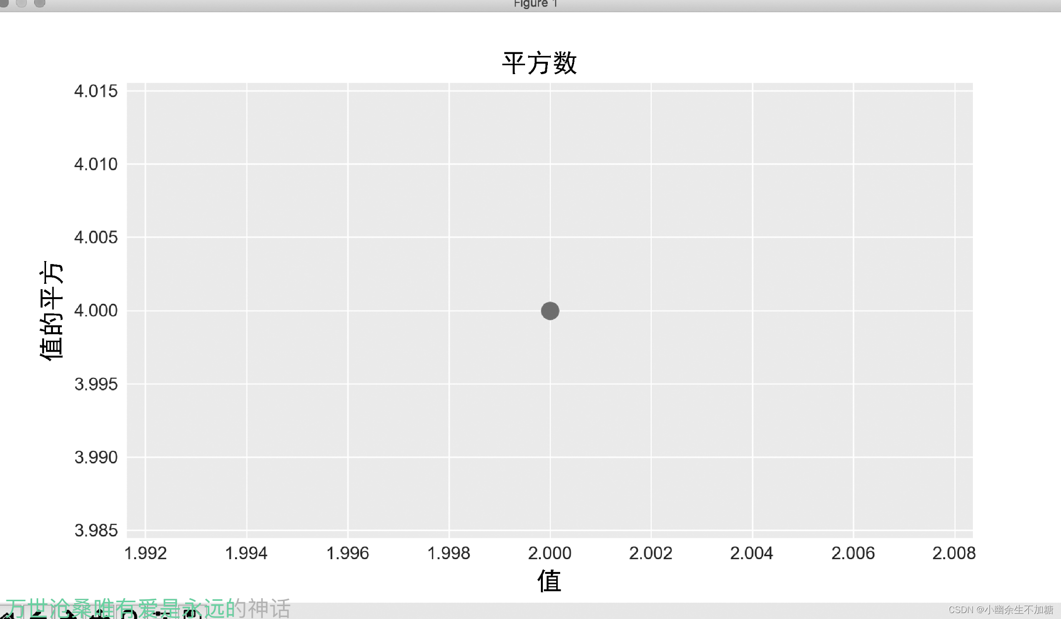
At ❶, call scatter() and use the parameter s to set the size of the points used when drawing the graph. If you run scatter_squares.py at this time, you will see a point in the center of the chart, as shown in the figure

2.5 Use scatter() to draw a series of points

To plot a series of points, pass scatter() two lists containing [inset] values ​​and [inset] values, as follows: scatter_squares.py

import matplotlib.pyplot as plt

x_values = [1, 2, 3, 4, 5]
y_values = [1, 4, 9, 16, 25]

plt.style.use('seaborn')
fig, ax = plt.subplots()
ax.scatter(x_values, y_values, s=100)

# 设置图表标题并给坐标轴指定标签。
--snip--

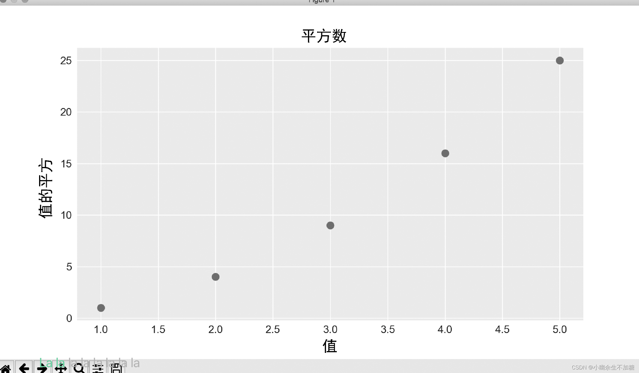
The list x_values ​​contains the numbers whose squares are to be calculated, and the list y_values ​​contains the squares of the aforementioned numbers. When these lists are passed to scatter(), Matplotlib reads a value from each list in turn to plot a point. The coordinates of the points to be drawn are (1, 1), (2, 4), (3, 9), (4, 16) and (5, 25), and the final result is shown in the figure.

2.6 Automatic calculation of data

Manually calculating the values ​​to include in the list can be inefficient, especially if there are many points to plot. We don't have to manually calculate the list containing the coordinates of the points, it can be done with a Python loop. Here is the code to draw 1000 points: scatter_squares.py

  import matplotlib.pyplot as plt

❶ x_values = range(1, 1001)
  y_values = [x**2 for x in x_values]

  plt.style.use('seaborn')
  fig, ax = plt.subplots()
❷ ax.scatter(x_values, y_values, s=10)

  # 设置图表标题并给坐标轴加上标签。
  --snip--

  # 设置每个坐标轴的取值范围。
❸ ax.axis([0, 1100, 0, 1100000])

  plt.show()

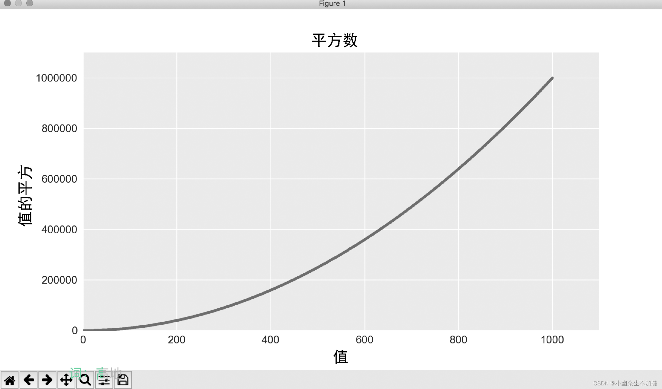
First, a list containing the values ​​of [Illustration] is created, which contains the numbers 1 to 1000 (see ❶). Next, is a list comprehension that generates the [illustration] values, iterates over the [illustration] values ​​(for xin x_values), computes their squared value (x**2), and stores the result into the list y_values. Then, pass the input list and output list to scatter() (see ❷). This dataset is large, so set the points to be small.

At ❸, use the method axis() to specify the value range of each coordinate axis. The method axis() requires 4 values: the [inset] and the minimum and maximum values ​​of the [inset] axis. Here, set the value range of the [Illustration] coordinate axis to 0~1100, and set the value range of the [Illustration] coordinate axis to 0~1 100 000. The result is shown in the figure.

2.7 Custom Colors

To modify the color of the data points, pass the argument c to scatter() and set it to the name of the color to use (in quotes), as follows:

ax.scatter(x_values, y_values, c='red', s=10)

Colors can also be customized using the RGB color mode. To specify a custom color, you can pass the parameter c and set it as a tuple containing three decimal values ​​from 0 to 1, representing the red, green and blue components respectively. For example, the following line of code creates a scatter plot of light green points:

ax.scatter(x_values, y_values, c=(0, 0.8, 0), s=10)

The closer the value is to 0, the darker the specified color; the closer the value to 1, the lighter the specified color.

2.8 Using colormaps

A colormap is a sequence of colors that fades from a starting color to an ending color. In visualizations, color maps are used to highlight regularities in data. For example, you might use a lighter color to show smaller values ​​and a darker color to show larger values.

The module pyplot has a set of colormaps built in. To use these colormaps, you need to tell pyplot how to color each point in the dataset. Here's how to set the color of each point based on its [inset] value:

scatter_squares.py

import matplotlib.pyplot as plt

x_values = range(1, 1001)
y_values = [x**2 for x in x_values]

ax.scatter(x_values, y_values, c=y_values, cmap=plt.cm.Blues, s=10)

# 设置图表标题并给坐标轴加上标签。
--snip--

We set the parameter c to a list of [illustration] values, and use the parameter cmap to tell pyplot which colormap to use. These codes display points with small values ​​of [inset] in light blue and points with high values ​​in [inset] in dark blue, as shown in the image.

2.9 Automatically save charts

To have the program automatically save the figure to a file, replace the call to plt.show() with a call to plt.savefig():

plt.savefig('squares_plot.png', bbox_inches='tight')

The first argument specifies what filename to save the graph with, this file will be stored in the same directory as scatter_squares.py. The second argument specifies that the extra white space of the chart should be cropped. If you want to preserve the extra white space around the chart, just omit this argument.