Article directory
1. Selection sort
Selection sort is the simplest and most intuitive sorting algorithm. Its principle is to loop through the unsorted data, find the smallest element in each round of traversal, and put it at the end of the sorted sequence. Regardless of the input data status, N rounds of traversal are required, so the time complexity is fixed O ( N 2 ) O(N^2)O ( N2 ). The advantage is that only a limited number of variables need to be applied, and the space complexity isO ( 1 ) O(1)O(1)。
code show as below:
/**
 * 选择排序
 * @param arr
 */
private static void selectionSort(int arr[]){


    for (int i = 0; i < arr.length-1; i++) {


        for (int j = i+1; j < arr.length; j++) {


            if(arr[j] < arr[i]){


                // 交换
                int temp = arr[i];
                arr[i] = arr[j];
                arr[j] = temp;
            }
        }
    }
}
2. Insertion sort
The basic idea of insertion sort is to insert a new element into an already sorted sequence. Similar to the process of constantly drawing and inserting cards into our hands when we play poker.
Its sorting process is as follows:
Traverse the array, assuming that the Kth element is currently reached, at this time the first 0~K-1 elements are already sorted, so only the Kth element and the K-1th element need to be compared, If the former is smaller than the latter, exchange the two elements and continue to traverse forward until the former is found to be larger than the latter.
code show as below:
/**
 * 插入排序
 * @param arr
 */
private static void insertionSort(int arr[]){


    for (int i = 0; i < arr.length; i++) {


        for (int j = i-1; j >=0 ; j--) {


            // 0~n 时,如果arr[n-1]>arr[n],则交换
            if(arr[j]>arr[j+1]){


                arr[j] = arr[j] ^ arr[j+1];
                arr[j+1] = arr[j] ^ arr[j+1];
                arr[j] = arr[j] ^ arr[j+1];
            } else {


                break;
            }
        }
    }
}
The time complexity of insertion sort is O ( N ) O(N) when the input data is sorted.O ( N ) , but stillO ( N 2 ) O(N^2)O ( N2 ). Its space complexity is alsoO ( 1 ) O(1)O(1)。
3. Bubble sort
Sort the elements in the sequence two by two. During the traversal process, the smaller elements will slowly float up like bubbles in water.
code show as below:
/**
 * 冒泡排序
 * @param arr
 */
private static void bubbleSort(int arr[]){


    for (int i = 0; i < arr.length; i++) {


        for (int j = 0; j < arr.length-1-i; j++) {


            if(arr[j] > arr[j+1]){


                int temp = arr[j];
                arr[j] = arr[j+1];
                arr[j+1] = temp;
            }
        }
    }
}
Fourth, merge sort
Merge sort is a typical application of divide and conquer algorithm. Its basic idea is to split the original sequence into small fragments, sort the small fragments first, then combine the fragments, and then sort them. In fact, it is a process from partial order to overall order.
The following shows the specific process through a specific example:

the code is as follows:
/**
 * 归并排序
 * @param arr 输入数据
 * @param L 左指针
 * @param R 右指针
 */
private static void process(int arr[],int L,int R){


    // base case
    if(L==R){


        return;
    }
    // 求出中点(其实就是(L+R)/2,先减后加防止溢出)
    int mid = L+((R-L)>>1);
    // 对左侧排序
    process(arr,L,mid);
    // 对右侧排序
    process(arr,mid+1,R);
    // 合并两边的子数组
    merge(arr,L,mid,R);
}

/**
 * 合并方法
 */
private static void merge(int arr[],int L,int M,int R){


    // 临时数组,用来存储排好序的一段数组元素,最后会拷贝回原数组
    int temp[] = new int[R-L+1];
    // 临时数组的指针
    int i = 0;
    // 左侧指针
    int p1 = L;
    // 右侧指针
    int p2 = M+1;
    // 左右两个指针所指元素进行比较,小的元素存入temp,它的指针向后移动
    while(p1<=M && p2<=R){


        temp[i++] = arr[p1]>arr[p2] ? arr[p2++]:arr[p1++];
    }
    // 当其中一个指针已经走完,说明另一半数组剩余的元素都比当前元素大
    // 所以将剩余的元素直接拷贝到临时数组
    while(p1<=M){


        temp[i++] = arr[p1++];
    }
    while(p2<=R){


        temp[i++] = arr[p2++];
    }
    // 最后再将临时数组拷贝回原数组
    for (int j = 0; j < temp.length; j++) {


        arr[L+j] = temp[j];
    }
}
According to Master formula T ( N ) = a ∗ T ( N / b ) + O ( N d ) T(N) = a*T(N/b) + O(N^d)T(N)=a∗T(N/b)+O ( Nd )It can be calculated that the time complexity of merge sorting isO ( N log N ) O(NlogN)O(NlogN)。
Five, quick sort
Quick sort is also a typical application of divide and conquer algorithm. We can introduce the basic idea of quick sort through an example:
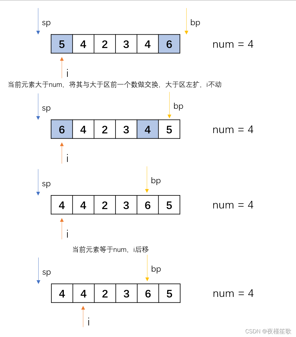
给定一个数组,和一个数num,要求将数组划分为左侧小于num,中间等于num和右侧大于num。
要求时间复杂度为O(N),空间复杂度为O(1)。
Since the required time complexity is O ( N ) O(N)O ( N ) , so the division of the array needs to be done in a finite number of traversals. You can consider maintaining two pointers to divide the array into greater than area, equal area and less than area. During the traversal, the movement of the two pointers represents the change of the boundaries of the greater than area and the less than area. Through these two pointers, we can know which elements are currently sorted and which elements are not yet sorted.
The following shows the specific process through an example:

code show as below:
/**
 * 荷兰国旗问题
 * @param arr 原数组
 * @param num 基准值
 */
private static void partition(int arr[],int num){


    int i = 0;
    // 小于区指针
    int smallPoint = -1;
    // 大于区指针
    int bigPoint = arr.length;
    while(i<bigPoint){


        // 小于时,当前元素与小于区下一个元素交换,小于区右扩
        if(arr[i] < num){


            int a = arr[smallPoint + 1];
            arr[smallPoint + 1] = arr[i];
            arr[i] = a;
            i++;
            smallPoint++;
        }else if(arr[i] == num){


            // 等于时,只动指针
            i++;
        }else{


            // 大于时,大于区前一个元素与当前元素互换,大于区左扩
            int a = arr[bigPoint - 1];
            arr[bigPoint - 1] = arr[i];
            arr[i] = a;
            bigPoint--;
        }
    }
}
Through the above example, we can find that after a round of partition processing, the elements equal to the area in the sequence have been arranged in their positions, that is, the elements in the front are all less than or equal to the elements in the area, and the elements in the back are all greater than or equal to the elements in the area. Then, if the above-mentioned processing is performed on the greater than area and the less than area, and recursively go down in turn, won't we be able to get an ordered sequence in the end? In fact, this is the basic idea of quick sort.

Quick sort uses a recursive strategy similar to merge sort, so the time complexity can also be derived from the Master formula as O ( N log N ) O(NlogN)O ( Nlog N ) , at the same time, the time complexity of quick sort on constant items is much smaller, so in general, the time complexity of quick sort is better than merge sort .
However, there is a problem with the above-mentioned version of quicksort. When faced with a sequence with a strong sequence, each time the reference number of a fixed position is selected, the partition will only have a greater than area and an equal area or only a less than area and an equal area. :

It is equivalent to only one element is arranged in each round of traversal, so the time complexity at this time isO ( N 2 ) O(N^2)O ( N2 ).
In order to optimize the performance of fast sorting in the worst case, we can change "select elements at fixed positions as the reference number each time" to "select elements at random positions as the reference number each time", so that although the time in each round of partition The complexity is uncertain, but overall the expected time complexity isO ( N log N ) O(NlogN)O ( Nl o g N ) .
code show as below:
/**
 * 快速排序
 *
 * @param arr 待排序数组
 * @param L 左边界
 * @param R 右边界
 */
private static void process(int arr[], int L, int R) {


    if (L >= R) {


        return;
    }
    // 随机位置的元素与最后一位元素交换
    swap(arr, (int) (L + Math.random() * (R - L + 1)), R);
    // 对当前序列进行划分
    int a[] = partition(arr, L, R);
    // 对大于区和小于区进行排序
    process(arr, L, a[0]);
    process(arr, a[1], R);
}

/**
 * 交换
 */
private static void swap(int arr[], int index1, int index2) {


    int a = arr[index1];
    arr[index1] = arr[index2];
    arr[index2] = a;
}

/**
 * 划分
 *
 * @param arr 要划分的数组
 * @param L 左边界
 * @param R 右边界
 * @return 小于区最后一个元素和大于区第一个元素
 */
private static int[] partition(int arr[], int L, int R) {


    // 小于区指针
    int smallPoint = L - 1;
    // 大于区指针
    int bigPoint = R;
    while (L < bigPoint) {


        // 当前数小于划分值,小于区下一个数与当前数交换,小于区右扩,L++
        if (arr[L] < arr[R]) {


            swap(arr, ++smallPoint, L++);
        } else if (arr[L] > arr[R]) {


            // 当前数大于划分值,大于区上一个数与当前数交换,大于区左扩
            swap(arr, --bigPoint, L);
        } else {


            // 当前数等于划分值,L++
            L++;
        }
    }
    // 最后,将划分值与大于区第一位元素交换
    swap(arr, R, bigPoint++);
    // 返回小于区末尾和大于区第一个元素
    return new int[]{

    smallPoint, bigPoint};
}
Six, heap sort
Heap sort is an algorithm that uses the data structure of the heap for sorting. The following two heaps are mainly used:
Large root heap: a complete binary tree in which each node is larger than its children.
Small root heap: A complete binary tree in which each node is smaller than its children.

So how is the heap generated? Let's take the big root heap as an example to explain:
Although the heap is a tree structure, we can use arrays to store it to improve its reading performance; Time complexity for adding and deleting operations. The heap structure mainly has the following two operations:
(1) Floating operation
When we insert an element into the heap, it is often inserted into the last position. At this time, the heap may no longer meet the characteristics of the big root heap, so we can Newly arrived nodes perform floating operations until the heap is adjusted back to the state of the large root heap. According to the characteristics of the large root heap—the root node is larger than all child nodes, we only need to compare the new node with its parent node when adjusting, and if it is larger than the parent node, exchange the two nodes until we encounter one larger than ourselves The parent node is stopped. current nodeThe parent node position of i also only needs to be obtained by calculation:( i − 1 ) / 2 (i-1)/2(i−1)/2。


code show as below:
/**
 * 上浮操作
 * @param arr 堆数组
 * @param index 要操作的元素下标
 */
private static void heapInsert(int arr[],int index){


    // 当前节点比父节点大,交换两者位置
    while(arr[index] > arr[(index-1)/2]){


        swap(arr,index,(index-1)/2);
        index = (index-1)/2;
    }
}
(2) Sinking operation
When we want to delete heap elements, we can add the last element of the heap to the top of the heap (generally, the heap will only delete the top element of the heap, and it is meaningless to delete other elements). At this time, the heap may lose the value of the big root heap. characteristics, so we need to perform a sinking operation on the new heap top node. You only need to compare it with your older child, and if it is smaller, exchange positions until you encounter a child node smaller than yourself.


code show as below:
/**
 * 下沉操作
 * @param arr 堆数组
 * @param index 要操作的元素下标
 * @param heapSize 堆大小
 */
private static void heapify(int arr[],int index,int heapSize){


    // 先拿到左孩子节点
    int left = index*2 + 1;
    while(left < heapSize){


        // 找到最大的孩子节点
        int largest = left+1 < heapSize && arr[left+1] > arr[left] ? left+1 : left;
        // 比较父节点与子节点
        largest = arr[index] > arr[largest] ? index : largest;
        // 如果父节点更大,退出循环
        if(largest == index){


            break;
        }
        // 子节点大,则交换父节点与子节点
        swap(arr,largest,index);
        // 继续向下寻找子节点
        index = largest;
        left = index*2+1;
    }
}
After mastering the above two heap adjustment methods, heap sorting is extremely simple. You only need to insert the original sequence into the heap (heapInsert) one by one, then take out the root node, and then adjust the remaining heap (heapify), and the cycle goes on and on. Until the data in the heap is fetched.
code show as below:
/**
 * 堆排序
 * @param arr 原数组
 */
private static void heapSort(int arr[]){


    // 转换成大根堆
    for (int i = 0; i < arr.length; i++) {


        heapInsert(arr,i);
    }
    // 堆大小
    int heapSize = arr.length;
    while(heapSize > 0){


        // 交换首尾元素,并断开尾元素与堆的链接
        swap(arr,0,--heapSize);
        // 对首元素进行下沉操作
        heapify(arr,0,heapSize);
    }
}

/**
 * 交换
 */
private static void swap(int arr[],int index1,int index2){


    int a = arr[index1];
    arr[index1] = arr[index2];
    arr[index2] = a;
}
Because both heapify and heapInsert operations only need to traverse the height of the heap, so the time complexity is O ( log N ) O(logN)O ( log N ) . _ _ During the sorting process, each element in the heap needs to be traversed, and a heapify operation will be performed every time an element is traversed, so the time complexity of heap sorting isO ( N log N ) O(NlogN)O(NlogN)。
Seven. Summary
Sorting stability: After a sorting, two elements that are originally equal still maintain the original order. Because in actual production, there is more than one dimension that affects the order of data, and it is often encountered that the attributes to be sorted are the same, but the original input order is not expected to be changed. Therefore, in some cases, whether the sorting algorithm is stable is also a standard for reference one.
Stable sorting algorithm: bubble sorting (no exchange when equal), insertion sorting (no exchange when equal), merge sorting (move the left pointer first when equal) unstable sorting algorithm: selection sort, quick sort, heap
sort
Finally, summarize the time, space complexity and stability of each algorithm:
| time complexity | space complexity | stability | |
|---|---|---|---|
| selection sort | O ( N 2 ) O(N^2)O ( N2) | O(1) O(1)O(1) | unstable |
| Bubble Sort | O ( N 2 ) O(N^2)O ( N2) | O(1) O(1)O(1) | Stablize |
| insertion sort | O ( N 2 ) O(N^2)O ( N2) | O(1) O(1)O(1) | Stablize |
| merge sort | O ( N l o g N ) O(NlogN) O(NlogN) | O ( N ) O(N)O ( N ) | Stablize |
| quick sort | O ( N l o g N ) O(NlogN)O(NlogN) | O ( l o g N ) O(logN) O(logN) | unstable |
| heap sort | O ( N l o g N ) O(NlogN)O(NlogN) | O(1) O(1)O(1) | unstable |