Learning Data Mining with Bank Marketing Data: Exploring Models to Predict Customer Purchase Behavior

0 understand the data

Source: UCI Machine Learning Repository ( https://archive.ics.uci.edu/ml/datasets/bank+marketing )

Dataset information:

This data relates to the direct marketing campaigns of Portuguese banking institutions. These marketing campaigns are based on phone calls. It is often necessary to contact the same customer several times to determine whether the product will be subscribed (term deposit in bank).

Attribute information:

Input variable:

1-age: age (numeric)

2-job: occupation type (category)

'admin.': administrative staff

'blue-collar': blue-collar worker

'entrepreneur': entrepreneur

'housemaid': housewife

'management': management personnel

'retired': retired person

'self-employed': Self-employed person

'services': service industry personnel

'student': student

'technician': technician

'unemployed': Unemployed people

'unknown': unknown occupation

3-marital: marital status (category)

'divorced': divorced or widowed

'married': married

'single': single

'unknown': unknown marital status

4-education: education level (category)

'basic.4y': 4 years of basic education

'basic.6y': 6-year basic education

'basic.9y': 9-year basic education

'high.school': high school education

'illiterate': illiterate

'professional.course': professional course education

'university.degree': undergraduate education

'unknown': unknown education level

5-default: default credit: is there a credit default? (category: 'no' no, 'yes' yes, 'unknown' unknown)

6-housing: Housing Loans: Is there a housing loan? (category: 'no' no, 'yes' yes, 'unknown' unknown)

7-loan: Personal Loan: Is there a personal loan? (category: 'no' no, 'yes' yes, 'unknown' unknown)

8-contact: contact method: contact communication type (category: 'cellular': mobile phone, 'telephone': telephone)

9- month: month: month of last contact of the year (category)

10- day_of_week: day of the week: last contact day of the week (category)

11-duration: duration: the duration of the last contact, in seconds (numeric). Important note: This property has a strong influence on the output target (e.g. y='no' if duration is 0). However, the duration is not known until the call is made. Also, y is obviously known after the call. Therefore, this input should only be included for benchmarking purposes, and discarded if the intent is to have a true predictive model.

12-campaign: Campaign: The number of contacts performed during this campaign and for this customer (numeric, including the last contact)

13-pdays: The number of days since the customer was last contacted from a previous campaign (numeric; 999 means the customer has not been contacted previously)

14-previous: Previous contacts: The number of contacts performed before this campaign and for this customer (numeric)

15-poutcome: results of previous marketing activities (categorical)

'failure': campaign failed

'nonexistent': no ​​previous campaign

'success': The campaign was successful

16-emp.var.rate: employment change rate - quarterly indicator (numeric)

17-cons.price.idx: Consumer Price Index - monthly indicator (numeric)

18-cons.conf.idx: consumer confidence index - monthly indicator (numeric)

19-euribor3m: Eurozone 3-month interval interest rate - daily indicator (numeric)

20-nr.employed: number of employees - quarterly index (numeric)

output variable:

y: Has the customer already subscribed to a term deposit? (binary: 'yes' yes, 'no no')

1 Import data

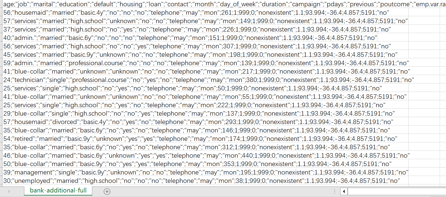
Read the data file named 'bank.csv' using the read_csv() method from the pandas library and save it in a DataFrame object named 'df'. The parameter 'encoding' specifies the encoding method of the data file as 'utf-8-sig', and the parameter 'sep' specifies the field separator in the data file as ';'.

Implementation code:

# 1 导入数据
df = pd.read_csv('bank-additional-full.csv', encoding='utf-8-sig', sep=';')
pd.set_option('display.max_columns', 100)  # 显示完整的列
# print(df.head(30))
# print(df.shape)

2 Data preprocessing

2.1 Numericalization of categorical data

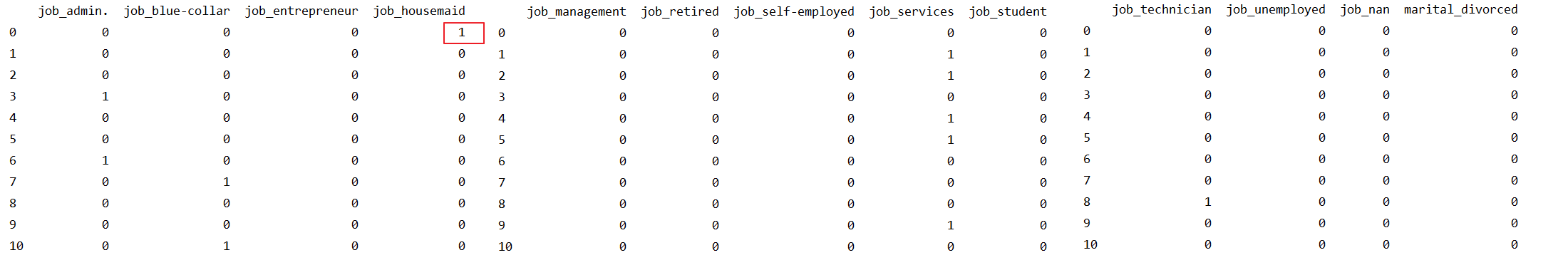
The categorical data here is divided into two cases, one is only contains two kinds of values ​​(except for the missing value of 'unknown', there are two kinds of values), and the other is the categorical data containing multiple values, such as education level (education ). For the first case, we can directly use 0 and 1 to replace the two values. For the second case, we can use dummy encoding or one-hot encoding to convert categorical data to numerical data, here, we use dummy encoding.

The processed data (part) is shown in the figure. We can see that for default, unknown is converted to NaN, and other values ​​are replaced by 0 and 1.

For the job, the result after we have performed the dummy encoding is shown in the figure below. We can see that the first piece of data is 000100000000, which means housemaid.

Implementation code:

def transform_to_binary(df, col_name):
    # yes->1   no -> 0   unknown -> NaN
    df[col_name] = df[col_name].map({'yes': 1, 'no': 0})  # 将"yes"值替换为1，将"no"值替换为0
    df[col_name].replace('unknown', np.nan, inplace=True)  # 将"unknown"替换为NaN
    return df

def dummy_variables(df, columns):
    # 哑编码
    for col in columns:
        # 将 "unknown" 替换为 NaN
        df[col] = df[col].replace('unknown', np.nan)
        # 进行哑编码
        dummies = pd.get_dummies(df[col], prefix=col, dummy_na=True)
        # 将原始列删除，并将编码列添加到 DataFrame 中
        df = df.drop(col, axis=1)
        df = pd.concat([df, dummies], axis=1)
    return df

# 2.1 分类数据数值化（哑编码）
categorical_columns = ['job', 'marital', 'education', 'default', 'housing', 'loan', 'contact', 'month', 'day_of_week',
                       'poutcome', 'y']  # 分类数据
numerical_columns = list(set(df.columns) - set(categorical_columns))  # 数值数据

# 二元分类数据
categoricaltobinarycols = ['default', 'housing', 'loan', 'y']
for col in categoricaltobinarycols:
    df = transform_to_binary(df, col)
# 分类数据哑编码
df = dummy_variables(df, ['job', 'marital', 'education', 'contact', 'month', 'day_of_week', 'poutcome'])

2.2 Numerical data normalization

数值型数据的规范化是指将数据缩放到指定的范围内，通常是将数据缩放到[0,1]或[-1,1]的区间内。进行规范化的原因是不同变量具有不同的量纲，这会影响机器学习算法的性能，导致一些变量对结果的贡献更大，而另一些变量对结果的贡献更小。Python中可以使用MinMaxScaler来进行规范化。

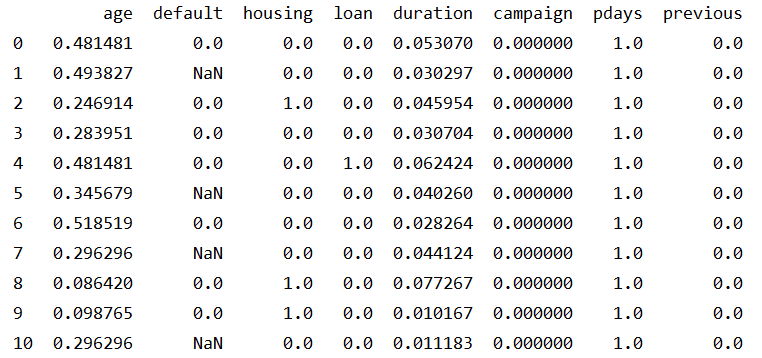
处理后数据如图，我们可以看出通过规范化可以将数值投射到[0,1]。

实现代码：

def normalize_columns(df, columns):
    # 进行规范化
    scaler = MinMaxScaler()
    for col in columns:
        if df[col].dtype != 'object':
            # 从 DataFrame 中提取出该列，并将其转换为二维数组
            col_data = df[[col]].values
            # 调用 MinMaxScaler 对象的 fit_transform() 方法进行规范化
            normalized_data = scaler.fit_transform(col_data)
            # 将规范化后的数组转换回一维，并将其添加回 DataFrame 中
            df[col] = normalized_data.flatten()
    return df

# 2.2 数值型数据标准化
df = normalize_columns(df, numerical_columns)

2.3 缺失值处理

我们需要检查数据中是否存在缺失值。数据中包含数值型数据和分类型数据。对于数值型数据（age，duration，campaign，pdays，previous，emp.var.rate，cons.price.idx，cons.conf.idx，euribor3m，nr.employed），我们可以使用 isnull() 方法来检查是否存在缺失值。对于分类型数据（），'unknown' 表示数据缺失，我们已将'unknown'替换为NaN，现使用isnull()方法进行统计。

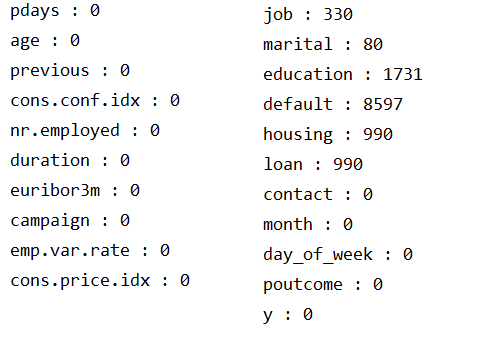
从结果可以看出，数值型数据没有缺失值，分类型中job, marital, education,default, housing, loan中存在缺失值。常见的缺失值处理方法如图所示：

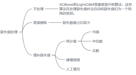
我们将目前存在缺失值的字段分为两种情况进行处理：

• 对于含有缺失值数据占比较小的字段（job 和 marital），我们可以直接删除这些缺失值所在的数据。

• 对于缺失值占比较大的字段（housing，loan，education和 default），我们可以使用不含缺失值的数据作为训练集，使用随机森林来预测缺失值，并用预测结果来填充缺失值。

实现代码：

# 2.3 缺失值处理

# 查看数值型属性缺失值
for col in numerical_columns:
     print(col + " : " + str(df[col].isnull().sum()))

 # 查看字符型属性缺失值
df.replace('unknown', np.nan, inplace=True)  #将"unknown"替换为NaN
for col in categorical_columns:
    print(col + " : " + str(df[col].isnull().sum()))


# 删除job和marital字段中的缺失值

job_cols = [col for col in df.columns if re.search('^job_', col)] # 使用正则表达式查找所有以 "job" 开头的列名
for col in job_cols:
    df.dropna(subset=[col], inplace=True)

marital_cols =[col for col in df.columns if re.search('^marital_', col)] # 使用正则表达式查找所有以 "marital" 开头的列名
for col in job_cols:
    df.dropna(subset=[col], inplace=True)

# 使用随机森林算法来预测缺失值
col_list = ['housing', 'loan', 'default']
education_cols = [col for col in df.columns if re.search('^education_', col)]
col_list += education_cols
df = impute_missing_values(df, col_list)

# 将经过处理后的 df 保存为 CSV 文件
df.to_csv('processed_data.csv', index=True)

3 模型建立

3.1 建模思路

对于银行营销数据，我们希望可以通过相关信息来确定客户是否会订阅产品（银行定期存款），即我们需要建立模型，使其可以根据输入变量（年龄，职业等）来预测输出变量（客户是否已经订阅定期存款），这是一个分类问题。

分类（classification）是指将数据按照某种标准或属性分成不同的类别或组别的过程。在分类问题中，数据通常被表示为特征（features）或属性（attributes），每个特征或属性具有一个值。分类的任务是对数据集进行学习并构造一个拥有预测功能的分类模型，用于预测未知样本的类标号。

以下是几种常用的分类方法：

• 决策树（Decision Tree）：通过树状结构来描述各种决策，其中每个叶节点表示一个类别，而非叶节点表示一个判断条件。

• 朴素贝叶斯（Naive Bayes）：基于贝叶斯定理的分类方法，它假设各个特征之间是相互独立的。

• 逻辑回归（Logistic Regression）：一种广义线性模型，适用于二元分类或多元分类。

• 支持向量机（Support Vector Machine）：通过构建最优超平面（或者多个最优超平面）来实现分类。

• 随机森林（Random Forest）：一种基于决策树的集成学习方法，通过多个决策树的投票来决定分类结果。

• K近邻算法（K-NearestNeighbor，KNN）：根据待分类数据点周围K个最近邻数据点的类别来判断该数据点所属的类别。

为了寻找最优模型，我们可以尝试多种不同的模型（例如逻辑回归、随机森林、支持向量机等），并对每个模型寻找最优模型参数。然后，将每个模型的预测结果与实际结果进行比较，选择表现最好的模型作为最终的模型。

3.2 划分数据集与重采样

在划分数据集时，通常将数据划分为训练集、验证集和测试集三个部分。划分比例的具体选择取决于具体的应用场景和数据量大小等因素，一般而言，通常按照 60%-20%-20% 或 70%-15%-15% 的比例进行划分，我们选择按照60%-20%-20%划分数据集。

训练集用于训练模型，确定模型的参数和结构。通常使用大部分数据作为训练集，以便使模型能够充分学习数据的特征和规律。验证集用于调整模型的超参数，如学习率、正则化参数等。在训练过程中，验证集的表现可以帮助我们选择最好的模型，并进行模型的调整，从而避免过拟合。测试集用于评估模型的泛化性能，检查模型是否过拟合或欠拟合。测试集应该是独立于训练集和验证集的，这样才能客观地评估模型的性能。

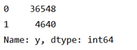
在对数据中输出变量y进行统计后发现，负样本（y=0）远多于正样本（y=1），负样本占大多数，这会导致模型的预测结果偏向负样本，而对于正样本的预测不够准确，从而影响了模型的准确性和可靠性。为减弱数据不均衡问题带来的不利影响，我们将采用重采样方法，重采样包括欠采样和过采样两种。

欠采样指的是从多数类（即负例）中删除一些样本，使得正例和负例的数量接近。欠采样可以减少数据量，提高训练速度，但是可能会造成信息损失，且如果欠采样不合理，可能会导致欠拟合的问题。

过采样指的是从少数类（即正例）中生成新的样本，使得正例和负例的数量接近。过采样可以增加数据量，提高模型的泛化性能，但是如果过采样不合理，可能会导致过拟合的问题。

我们将使用SMOTE实现过采样以平衡数据，SMOTE（Synthetic Minority Over-samplingTechnique）是根据少数类样本之间的相似性生成新的样本，以达到平衡数据集的目的。具体来说，SMOTE算法的步骤如下：

1.对于每个少数类样本，计算其与所有少数类样本之间的欧氏距离，并将距离最近的K个样本记录下来，这些样本称为其K近邻样本。

2.对于每个少数类样本，从其K近邻样本中随机选择一个样本，然后在少数类样本与该样本之间的连线上随机生成一个新的样本，即生成的新样本的每个特征值都是原始样本和该K近邻样本对应特征值的线性插值。

3.将生成的新样本添加到原始的少数类样本集中，从而构成一个新的平衡的数据集。

实现代码：

#划分数据集
train_data, test_val_data = train_test_split(df, test_size=0.4,
                                             random_state=42)  # 使用train_test_split函数将原始数据集data按照test_size=0.4的比例划分为训练集train_data和测试集+验证集的组合test_val_data，其中test_size表示测试集所占比例，这里设置为40%。
test_data, val_data = train_test_split(test_val_data, test_size=0.5,
                                       random_state=42)  # 使用train_test_split函数将test_val_data按照test_size=0.5的比例划分为测试集test_data和验证集val_data
# 打印数据集大小
print(f'Train data size: {train_data.shape[0]}')
print(f'Validation data size: {val_data.shape[0]}')
print(f'Test data size: {test_data.shape[0]}')

# 简单统计查看数据是否平衡
print(df['y'].value_counts())

# 对训练集数据进行SMOTE

X_train = train_data.drop("y", axis=1)
y_train = train_data["y"]

smote = SMOTE(random_state=42, k_neighbors=3)
X_train_res, y_train_res = smote.fit_resample(X_train, y_train)
print('原始数据集中各类别样本数量：\n', y_train.value_counts())
print('过采样后数据集中各类别样本数量：\n', y_train_res.value_counts())

X_train_res = X_train_res.values
y_train_res = y_train_res.values

X_test = test_data.drop("y", axis=1).values
y_test = test_data["y"].values

X_val = val_data.drop("y", axis=1).values
y_val = val_data["y"].values

3.3 模型的训练与评估

常见的分类模型包括逻辑回归（Logistic Regression）、决策树（Decision Tree）、随机森林（Random Forest）、朴素贝叶斯（Naive Bayes）、支持向量机（Support Vector Machine,SVM）、K近邻算法（K-Nearest Neighbors）、神经网络（Neural Networks）等。我们将选择逻辑回归、朴素贝叶斯、支持向量机和随机森林在训练集上进行训练，并分别进行参数寻优，在交叉验证集上进行评估，随机森林表现更优，所以最终选择在随机森林模型在测试集上进行测试。

通过网格调参得到各模型在训练集上的最优参数：

逻辑回归：

朴素贝叶斯：

随机森林：

使用各模型最佳参数对训练集数据进行训练，并在交叉验证集上进行测试，打印各模型正样本的f1-score：

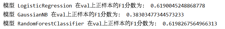
最后，我们将选择f1得分最高的随机森林模型进行应用，打印正样本的f1-score：

实现代码：

# 3.0 定义评价指标为正样本的F1-score
scoring = {'f1_score': make_scorer(f1_score, pos_label=1)}

#3.1在训练集上建立逻辑回归模型(Logistic Regression)，并寻找最优参数

# 创建Logistic Regression对象
lr_model = LogisticRegression(max_iter = 100000)

# 定义要搜索的参数组合
parameters_lr = {
    'solver': ['lbfgs', 'liblinear'],
    'penalty': ['l1', 'l2'],
    'C': [0.1, 1, 10]
}

# 创建GridSearchCV对象
grid_search_lr = GridSearchCV(lr_model, parameters_lr, scoring=scoring, cv=5, return_train_score=True, refit='f1_score')

# 在训练集上拟合GridSearchCV对象
grid_search_lr.fit(X_train_res, y_train_res)

# 输出最优参数及其对应的分数
print("Model name: Logistic Regression")
print("Best parameters: ", grid_search_lr.best_params_)
print('Best Score:', grid_search_lr.best_score_)

#3.2在训练集上建立朴素贝叶斯模型(Naive Bayes)，并寻找最优参数

# 设置参数范围
parameters_clf = {
    'var_smoothing': np.logspace(0,-9, num=100)
}

# 创建一个GaussianNB分类器对象
clf = GaussianNB()

# 创建GridSearchCV对象
grid_search_clf = GridSearchCV(clf, parameters_clf, scoring=scoring, cv=5,return_train_score=True, refit='f1_score')

# 在训练集上拟合GridSearchCV对象
grid_search_clf.fit(X_train_res,y_train_res)

# 打印最优参数和最优得分
print("Model name: Naive Bayes")
print("Best parameters: {}".format(grid_search_clf.best_params_))
print("Best F1-score: {:.2f}".format(grid_search_clf.best_score_))

#3.3在训练集上建立随机森林模型(Random Forest)，并寻找最优参数

# 定义参数范围
parameters_rfc = {'n_estimators': [50, 100, 200],
          'max_depth': [5, 10, 20],
          'min_samples_split': [2, 5, 10],
          'min_samples_leaf': [1, 2, 4]}

# 创建模型
rfc = RandomForestClassifier()

# 创建GridSearchCV对象
grid_search_rfc = GridSearchCV(estimator=rfc, param_grid=parameters_rfc, scoring=scoring, cv=5,return_train_score=True, refit='f1_score')

# 在训练集上拟合GridSearchCV对象
grid_search_rfc.fit(X_train_res,y_train_res)

# 输出最优参数和最优得分
print("Model name: Random Forest")
print('Best parameters:', grid_search_rfc.best_params_)
print('Best score:', grid_search_rfc.best_score_)

#4 在交叉验证集上测试各模型的性能
best_lr_model = LogisticRegression(C=0.1, penalty='l1', solver='liblinear', max_iter=100000)
best_clf_model = GaussianNB(var_smoothing=1.519911082952933e-06)
best_rfc_model= RandomForestClassifier(max_depth =20,min_samples_leaf=1,min_samples_split=2,n_estimators = 100)

models = [best_lr_model, best_clf_model, best_rfc_model]

best_lr_model.fit(X_train_res,y_train_res)
best_clf_model.fit(X_train_res,y_train_res)
best_rfc_model.fit(X_train_res,y_train_res)

for model in models:
    y_pred = model.predict(X_val)
    f1 = f1_score(y_val, y_pred, pos_label=1)
    print("模型", model.__class__.__name__, "在val上正样本的F1分数为：", f1)

#5 在测试集上应用随机森林 RandomForestClassifier
y_pred_test = best_rfc_model.predict(X_test)
f1 = f1_score(y_test, y_pred_test, pos_label=1)
print("模型", model.__class__.__name__, "在测试集上正样本的F1分数为：", f1)

4 展望

最终建立的随机森林模型还有提高的可能性，我们可以考虑以下几个方面来提高F1得分：

• 特征工程：通过选择更好的特征或者构造新的特征，使得模型更能捕捉样本之间的差异和关联，提高模型的分类性能。

• 模型集成：将多个模型进行集成，可以获得更好的分类性能，如投票、平均、加权平均等集成方法。

• 模型选择：尝试使用其他算法或者改进的模型结构，如神经网络、深度学习等，以期获得更好的分类性能。