Implementation and model building of convolution and pooling in Pytorch

In the previous article, the use of some methods in the Dataset class and Transform class in Pytorch has been introduced. Next, the implementation of convolution and other operations using Pytorch will be introduced.

1. nn.Module class

A nn.Module is the basic skeleton of a neural network and can be viewed as a block. If the neural network needs to override the initialization method, it must call the initialization function of the parent class.

All modules contain two main functions:

init function: define some required classes or parameters in it. Including the network layer.

forward function: do the final calculation and output, and its formal parameter is the input of the model (block).

Now let's simply write a class:

class Test1(nn.Module):
    def __init__(self) -> None:
        super().__init__()

    def forward(self,input):
        output = input+1
        return output

The function of this class is to pass in a number, output the result of adding one to the number, and call the class:

test1 = Test1()

x = torch.tensor(1.0)

Note: There is no need to refer to the function when calling the forward method, because the forward method in the integrated nn.Module is the implementation of the __call__() method, and the callable object will call the __call__() method.

output = test1(x)

print(output)

The output is as follows:

 

Two, convolution

1、conv2d

The convolution integral is divided into different layers, such as con1, con2, etc. Taking the two-layer convolution as an example, the specific parameters can be found in the official document. The convolution operation is mainly calculated with the convolution kernel (weight) and the original data, plus Other operations, and finally get a new output. .

The meanings of some of these important parameters are as follows:

output is the calculated output of the convolutional neural network model.

input is the input data, here it is a two-dimensional array representing a picture.

Kernel represents the convolution kernel. It is also a two-dimensional array like the input shape, and both shapes must have four indicators, otherwise reshape is required.

stride represents the step size.

padding indicates how many layers are filled around, and the default value of padding is 0.

First import the package:

import torch

import torch.nn.functional as F

Set input data:

input = torch.tensor([[1, 2, 0, 3, 1],

                      [0, 1, 2, 3, 1],

                      [1, 2, 1, 0, 0],

                      [5, 2, 3, 1, 1],

                      [2, 1, 0, 1, 1]])

Set the convolution kernel:

kernel = torch.tensor([[1, 2, 1],

                       [0, 1, 0],

                       [2, 1, 0]])

Because the set data is incomplete, reshape is performed

input = torch.reshape(input, (1, 1, 5, 5))

kernel = torch.reshape(kernel, (1, 1, 3, 3))

Perform a convolution with a stride of 1:

output1 = F.conv2d(input, kernel, stride=1)

print(output1)

The output is as follows:

 

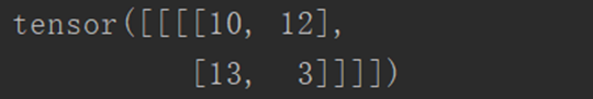
Perform a convolution with a stride of 2:

output2 = F.conv2d(input, kernel, stride=2)

print(output2)

The output is as follows:

 

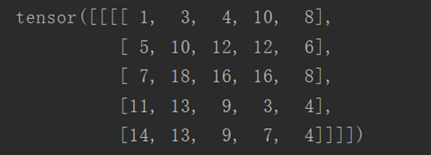
Perform a convolution with a step size of 1 and a padding layer of 1:

output3 = F.conv2d(input, kernel, stride=1, padding=1)

print(output3)

The output is as follows:

 

2、Conv2d

In fact, it is a further encapsulation of nn.function, such as nn.Conv2(), the most commonly used are these five parameters: in_channels, out_channels, kernel_size, stride, padding

First import the required packages:

import torch

import torchvision

from torch import nn

from torch.nn import Conv2d

from torch.utils.data import DataLoader

from torch.utils.tensorboard import SummaryWriter

Use dataset to download the required training samples, and use dataloader to package:

dataset = torchvision.datasets.CIFAR10('dataset', train=False, transform=torchvision.transforms.ToTensor(),download=True)

dataloader = DataLoader(dataset, batch_size=64)

Construction class:

class Test1(nn.Module): 

    def __init__ ( self ): 

        super (Test1 , self ). __init__ () 

        #Because it is a color image, so in_channels=3, the number of output channels=6 

        self .conv1 = Conv2d( in_channels = 3 , out_channels = 6 , kernel_size = 3 , stride = 1 , padding = 0 ) 



    def forward ( self , x): 

        x = self .conv1(x)

        return x

At this point, the set convolution kernel size is 3x3, and the number of output channels is 6.

Call the class, pass the training sample into the class, and display it in the browser:

test1 = Test1()

step = 0

writer = SummaryWriter('logs_conv2d')

for data in dataloader:

    imgs, targets = data

    output = test1(imgs)

#Incoming image before convolution, torch.Size([64, 3, 32, 32]) 

    writer.add_images( 'iuput' , imgs , step) 

    #Incoming image after convolution, torch.Size([64 , 6, 30, 30]) 

    # The number of channels of the image after convolution is 6, and the image cannot be displayed 

    output = torch.reshape(output , (- 1 , 3 , 30 , 30 )) 

    writer.add_images( 'output' , output , step) 

    step = step + 1 

writer.close()

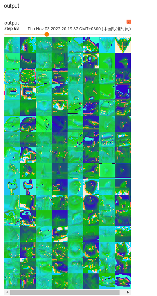
The output is as follows:

Input is the original image:

Output is the convolved image:

 

3. Maximum pooling

The role of the maximum pooling layer (commonly used is maxpool2d):

One is to further reduce the dimensionality of the information extracted by the convolutional layer and reduce the amount of calculation.

The second is to strengthen the invariance of image features, so as to increase the robustness of image offset and rotation.

The third is similar to the different resolutions when watching a video, the actual effect is like mosaicing a picture.

1. Maximum pooling of two-dimensional arrays

First import the package:

import torch

from torch import nn

from torch.nn import MaxPool2d

Define a binary tensor-like array:

input = torch.tensor([[1, 2, 0, 3, 1],

                      [0, 1, 2, 3, 1],

                      [1, 2, 1, 0, 0],

                      [5, 2, 3, 1, 1],

                      [2, 1, 0, 1, 1]], dtype=torch.float32)

Perform reshape:

input = torch.reshape(input, (-1, 1, 5, 5))

Define the class for max pooling:

class Test1(nn.Module):

    def __init__(self):

        super(Test1, self).__init__()

        self.maxpool1 = MaxPool2d(kernel_size=3, ceil_mode=True)



    def forward(self, input):

        output = self.maxpool1(input)

        return output

Above, when the filter is 3x3 and ceil_mode is True, redundant pixels are not discarded, and zeros are added to the original array that does not satisfy 3x3.

Call class:

test1 = Test1()

output = test1(input)

print(output)

The output is as follows:

2. Perform maximum pooling on the image

First import the package:

import torchvision

from torch import nn

from torch.nn import MaxPool2d

from torch.utils.data import DataLoader

from torch.utils.tensorboard import SummaryWriter

Use dataset to download the required training samples, and use dataloader to package:

dataset = torchvision.datasets.CIFAR10('dataset', train=False, transform=torchvision.transforms.ToTensor(),download=True)

dataloader = DataLoader(dataset, batch_size=64)

Construction class:

class Test1(nn.Module):

    def __init__(self):

        super(Test1, self).__init__()

        self.maxpool1 = MaxPool2d(kernel_size=3, ceil_mode=True)

    def forward(self, input):

        output = self.maxpool1(input)

        return output

Call class:

test1 = Test1()

step = 0

writer = SummaryWriter('logs_maxpool')

for data in dataloader:

    imgs, targets = data

    output = test1(imgs)

    writer.add_images('iuput', imgs, step)

    writer.add_images('output', output, step)

    step = step + 1


writer.close()

The output is as follows:

The original image is as follows:

 

The image after max pooling is as follows:

 

4. Nonlinear activation

The main purpose of non-linear transformation is to add some non-linear features to the network. The more non-linear, the more the model can be trained to meet various characteristics. Common non-linear activations:

ReLU: It is mainly to truncate what is less than 0 (turning what is less than 0 to 0), and the effect of image transformation is not obvious. The main parameter is inplace:

When inplace is true, assign the processed result to the original parameter; when it is false, the original value will not change.

Sigmoid: Normalized processing. The effect is not as good as ReLU, but for the problem of how far to classify, sigmoid must be used.

Take the ReLU method as an example:

First import the package

import torch

from torch import nn

from torch.nn import ReLU

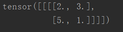
Set incoming parameters:

input = torch.tensor([[1, -0.5],

                      [-1, 3]])

input = torch.reshape(input, (-1, 1, 2, 2))

Construction class:

class Test1(nn.Module):

    def __init__(self):

        super(Test1, self).__init__()

        self.relu1 = ReLU()

    def forward(self, input):

        output = self.relu1(input)

        return output

Call class:

test1 = Test1()

output = test1(input)

print(output)

The output is as follows:

 

5. Linear layer

The linear layer is also called a fully connected layer, in which each neuron is connected to all neurons in the previous layer.

The linear function is: torch.nn.Linear(in_features, out_features, bias=True, device=None, dtype=None), and the three important parameters in_features, out_features, and bias are described as follows:

in_features: the size of the features for each input (x) sample

out_features: the size of the features for each output (y) sample

bias: If set to False, the layer will not learn additional bias. The default value is True, which means to increase the learning bias.

    In the figure above, in_features=d, out_features=L.

The effect can be to reduce the length of one-dimensional data.

• Use of Sequential (torch.nn.Sequential)

All required operations can be written in one function. It is mainly to facilitate the writing of code and make the code more concise.

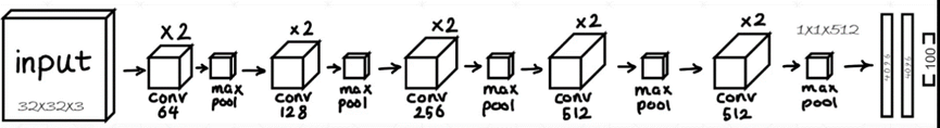
For example, implement the model shown in the figure below:

 

First import the package:

import torch

from torch import nn

from torch.nn import Conv2d, MaxPool2d, Flatten, Linear, Sequential

from torch.utils.tensorboard import SummaryWriter

Construction class:

class Test(nn.Module):

    def __init__(self):

        super(Test, self).__init__()

        self.model1 = Sequential(

            Conv2d(in_channels=3, out_channels=32, kernel_size=5, stride=1, padding=2),

            MaxPool2d(2),

            Conv2d(in_channels=32, out_channels=32, kernel_size=5, padding=2, stride=1),

            MaxPool2d(2),

            Conv2d(in_channels=32, out_channels=64, kernel_size=5, padding=2, stride=1),

            MaxPool2d(2),

            Flatten(),

            Linear(in_features=1024, out_features=64),

            Linear(in_features=64, out_features=10)

        )



    def forward(self, x):

        x = self.model1(x)

        return x

Call class:

test1 = Test()

print(test1)

input = torch.ones((64, 3, 32, 32))

output = test1(input)

print(output.shape)



writer = SummaryWriter('logs_seq1')

writer.add_graph(test1, input)

writer.close()

The output is as follows:

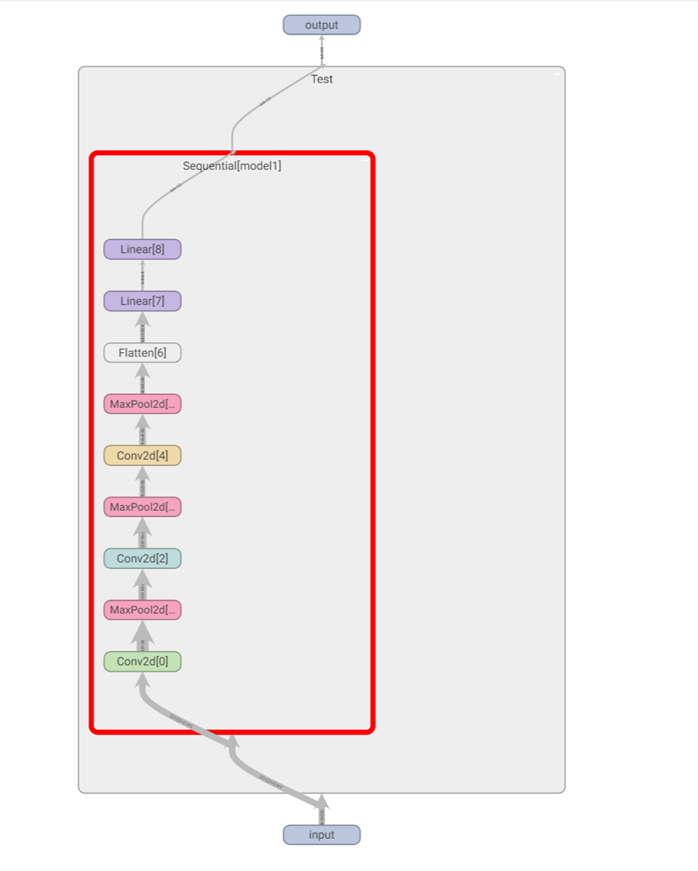
 You can see the context of this neural network model.