Modern Recurrent Neural Networks: Bidirectional Recurrent Neural Networks

Column: Neural Network Recurrence Directory

bidirectional recurrent neural network

Bidirectional Recurrent Neural Network (BRNN for short) is a neural network capable of processing sequence data, which can simultaneously consider past and future information in a sequence of data. Unlike traditional recurrent neural networks (RNNs), BRNNs use two separate recurrent structures at each time step, one for passing information from the past to the future and the other for passing information from the past to the past .

The main idea of ​​BRNN is to process the input sequence from two directions (forward and backward) separately, and then combine their outputs. In this way, BRNN can utilize all the information in the sequence, including past and future, so as to better capture the long-term dependencies in the sequence. For example, in natural language processing, BRNN can process left-to-right and right-to-left text sequences, improve the quality of text representation, and thus improve the performance of the model.

---

---

Dynamic Programming in Hidden Markov Models

Hidden Markov Model (HMM) is a probabilistic model for modeling sequence data, which is often used in speech recognition, natural language processing, bioinformatics and other fields. HMM assumes that each observation data is composed of a hidden state sequence and a state-related observation sequence. Among them, the hidden state sequence is a Markov process, that is, each state is only related to the previous state. An observation sequence is a sequence of observation data generated by each state.

In HMM, the forward algorithm and the backward algorithm are usually used to calculate the probability of a given observation sequence. Both algorithms are solved using dynamic programming.

The forward algorithm is used to calculate the observation sequence $O=(o_1,o_2,...,o_T)$ shape$l=(p,A,B)$ under the probability$P(O|\lambda )$ . Its basic idea is that at each time step$t$ , calculate all observations in the known previous values$o_1,o_2,...,o_{t-1}$In the case of , the system is in state iiProbability of$i$$a_t\left(i\right)$ . This probability can be calculated recursively. Specifically, for$t=1$ , we have
$$a_1(i)={Pi}_i{b}_i(o_1)$$

for $t>1$，我们有
$$a_t\left(i\right)=\left[\sum _{j=1}^N{a}_{t-1}\left(j\right){has}_{ji}\right]b_i\left(o_t\right)$$

Among them, $N$ is the number of hidden states,$a_{ij}$Indicates from state $i$ transitions to state$The\; probability\; of\; j$ ,$b_i(o_t)$ means that in state$i$ generate observation$o_t$The probability.

Calculate α t ( i ) \alpha_t(i) by recursion$a_t\left(i\right)$ , we can finally get$P(O|\lambda )={\sum }_{i=1}^N{a}_T(i)$。

The backward algorithm is used to calculate the given observation sequence $O$ and model$Under\; \lambda$ , the system is in stateiiProbability of$i$$b_t\left(i\right)$ . The basic idea of ​​the backward algorithm is to know all observations$o_{t+1},o_{t+2},...,o_T$In the case of , the system is in state $probability\; of\; i$ . Specifically, for$t=T$ , we have
$$b_T(i)=1$$

for $t<T$，我们有
$$b_t\left(i\right)=\sum _{j=1}^N{a}_{ij}{b}_j(o_{t+1})b_{t+1}(j)$$

Calculate β t ( i ) \beta_t(i) by recursion$b_t\left(i\right)$ , possible$P(O|\lambda )={\sum }_{i=1}^N{Pi}_i{b}_i(o_1)b_1(i)$。

At the same time, the forward algorithm and the backward algorithm can also be used to calculate the given observation sequence and model, the system is in a certain state iiThe probability of$i$$c_t\left(i\right)$ and from state$i$ to statejjThe transition probability of$j$$X_t(i,j)$ . Specifically, for$t=1,2,...,T$ , we have

$$c_t(i)=\frac{a_t\left(i\right)b_t(i)}{P(O|\lambda )}$$

$$X_t(i,j)=\frac{a_t(i)a_{ij}{b}_j(o_{t+1})b_{t+1}(j)}{P(O|\lambda )}$$

Among them, $P(O|\lambda )$ is the observation sequence$O$ in the modelλ \lambdaThe probability under$\lambda \; .$

The application of dynamic programming in HMM allows us to efficiently calculate the probability of the observation sequence, as well as the probability and transition probability of the system in a certain state given the observation sequence. This is very helpful for both model training and prediction.

two-way model

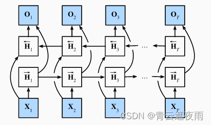
If we want to have a mechanism in the recurrent neural network that can provide similar forward-looking capabilities as hidden Markov models, we need to modify the design of the recurrent neural network. Fortunately, this is conceptually easy, just adding a RNN that "runs backwards from the last token" instead of just a "starting from the first token" in forward mode running" recurrent neural network. Bidirectional RNNs add hidden layers that pass information backwards in order to process such information more flexibly. The diagram below depicts the architecture of a bidirectional recurrent neural network with a single hidden layer.

mathematical definition

Forward hidden state:
$$H_{\to t}=\varphi (X_t{W}_{xh}+H_{\to t-1}{W}_{hh}+b_h)$$
reverse hidden state:
$$H_{\leftarrow t}=\varphi (X_t{W}_{xh}+H_{\leftarrow t+1}{W}_{hh}+b_h)$$
Export:
$$O_t=H_t{W}_{hq}+b_q$$
Among them, $X_t$Come in, $W_{xh},W_{hh},W_{hq}$is the weight matrix, $b_h,b_q$is a bias term, $\varphi$ is the activation function,$H_{\to t}$和 $H_{\leftarrow t}$are the forward and reverse hidden states, $H_t=[H_{\to t};H_{\leftarrow t}]$ is a two-way hidden state,$O_t$is the output.

The Computational Cost of the Model and Its Application

A key property of bidirectional recurrent neural networks is that they use information from both ends of the sequence to estimate the output. That is, we use information from past and future observations to predict current observations. But in the case of predicting the next token, such a model is not what we need. Because when predicting the next token, we can't know what the next token will be after all, so we won't get good accuracy. Specifically, during training, we are able to use past and future data to estimate the present vacant word; while during testing, we only have past data, so the accuracy will be poor. The following experiment will illustrate this point.

Another serious problem is that bidirectional recurrent neural networks are computationally very slow. The main reason is that the forward propagation of the network requires forward and backward recursion in the bidirectional layer, and the backward propagation of the network also depends on the result of the forward propagation. Therefore, the gradient solver will have a very long chain.

defect! !

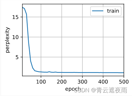
Since bidirectional recurrent neural networks use past and future data, we cannot blindly apply this language model to any prediction task. Although the perplexity levels produced by the model are reasonable, the model's ability to predict future tokens may be severely flawed. We use the sample code below as a warning in case they are used in the wrong context.

import torch
from torch import nn
from d2l import torch as d2l

# 加载数据
batch_size, num_steps, device = 32, 35, d2l.try_gpu()
train_iter, vocab = d2l.load_data_time_machine(batch_size, num_steps)
# 通过设置“bidirective=True”来定义双向LSTM模型
vocab_size, num_hiddens, num_layers = len(vocab), 256, 2
num_inputs = vocab_size
lstm_layer = nn.LSTM(num_inputs, num_hiddens, num_layers, bidirectional=True)
model = d2l.RNNModel(lstm_layer, len(vocab))
model = model.to(device)
# 训练模型
num_epochs, lr = 500, 1
d2l.train_ch8(model, train_iter, vocab, lr, num_epochs, device)