Table of contents
1.1 Difficulties in using Transformer in the visual field
1.2 Improvement of input sequence length
I. Introduction
1.1 Difficulties in using Transformer in the visual field
In NLP, the input to the transformer is a sequence, but in the visual field, it is necessary to consider how to convert a 2D image into a 1D sequence. The most intuitive idea is to input the pixels in the image into the transformer, but this will There is a problem, because the size of the picture in the model training is 224*224=50176, and the sequence length of the normal Bert is 512, which is 100 times that of Bert. The complexity of this is too high.
1.2 Improvement of input sequence length
If the complexity of directly inputting pixels is too high, think about how to reduce the complexity of this part
1) Use the feature map in the middle of the network
For example, the feature map size of the last stage res4 of res50 is only 14*14=196, and the sequence length meets expectations
2) Isolated self-attention
Using the local window instead of the entire graph, the length of the input sequence can be controlled by the windows size
3) Axis self-attention
Changing the self-attention operation on the 2D image to self-attention in the two dimensions of the height and width of the image can greatly reduce the complexity, but since the current hardware does not accelerate this operation, it is difficult to support large The magnitude of the data scale.
1.3 VIT Improvements to Input
First divide the image into patches, and then each patch is input into the transformer as a token. However, since the entire transformer will perform attention between each token, there is no order problem in the input itself. But for pictures, there is an order between each patch, so analogy to bert, add a position embedding (sum) to each patch embedding. At the same time, the final output also borrows from bert, replacing the whole with 0 and cls, and the corresponding embedding of this part is the final output.
2. Vision Transformer model
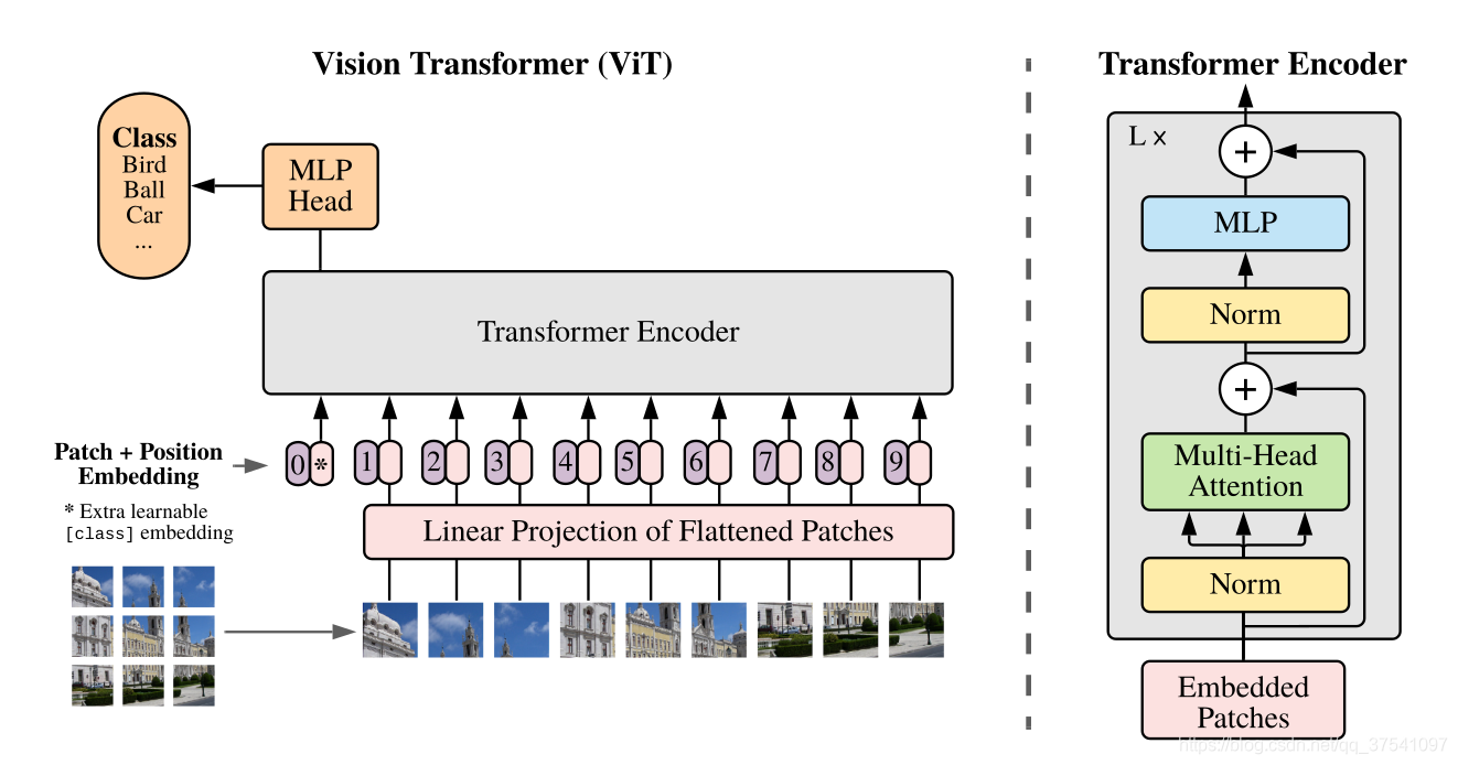
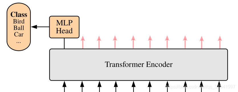
The figure below is the model framework of Vision Transformer (ViT) given in the original paper. In simple terms, the model consists of three modules:
1.Linear Projection of Flattened Patches(Embedding层)
2.Transformer Encoder
3.MLP Head (final layer structure for classification)
2.1 Embedding layer
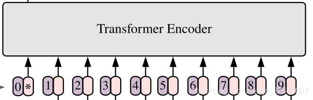
For the standard Transformer module, the required input is a token (vector) sequence, that is, a two-dimensional matrix [num_token, token_dim], as shown in the figure below, token0-9 corresponds to a vector, taking ViT-B/16 as an example, each token The vector length is 768.
For image data, its data format is [H, W, C], which is a three-dimensional matrix, which is obviously not what Transformer wants. Therefore, it is necessary to transform the data through an Embedding layer first. As shown in the figure below, first divide a picture into a bunch of Patches according to a given size. Taking ViT-B/16 as an example, the input image (224x224) is divided into patches of 16x16 size, and 196 Patches will be obtained after division. Then each Patch is mapped to a one-dimensional vector through linear mapping. Taking ViT-B/16 as an example, the shape of each Patch data is [16, 16, 3] and a vector with a length of 768 is obtained through mapping (the following are directly called token). [16, 16, 3] -> [768]
In the code implementation, it is implemented directly through a convolutional layer. Taking ViT-B/16 as an example, it directly uses a convolution with a convolution kernel size of 16x16, a step size of 16, and a convolution kernel number of 768. Through convolution [224, 224, 3] -> [14, 14, 768], and then flatten the two dimensions of H and W [14, 14, 768] -> [196, 768], it is just right at this time It becomes a two-dimensional matrix, which is exactly what Transformer wants.
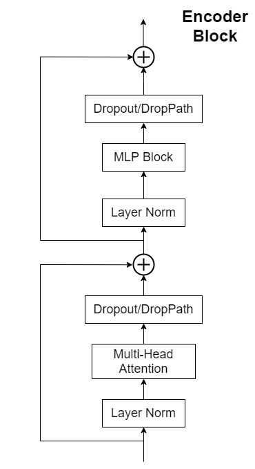
2.2 Transformer Encoder
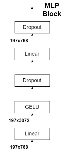
Transformer Encoder is actually stacking Encoder Block L times repeatedly, mainly composed of Layer Norm, Multi-Head Attention, Dropout and MLP Block.
2.3 MLP Head
The output shape and the input shape after passing the Transformer Encoder above remain unchanged. Take ViT-B/16 as an example, whether the input is [197, 768] or [197, 768]. Here we only need classification information, so we only need to extract the corresponding result generated by [class]token, that is, extract [1, 768] corresponding to [class]token from [197, 768]. Then we get our final classification result through MLP Head. In the original paper of MLP Head, it is said that when training ImageNet21K, it is composed of Linear+tanh activation function+Linear. But when migrating to ImageNet1K or your own data, only one Linear is enough.
2.4 Specific process
1. First, the input video with a resolution of T × H × W, where T is the number of frames, H is the height, and W is the width, is divided into non-overlapping blocks with a size of 1×16×16, and then on the flat image block Apply a linear layer point by point, projecting it into latent dimension D. It is the convolution of the kernel size and step size of 1×16×16, as shown in the patch1 stage in Table 1.
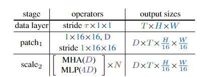
2. A positional embedding E ∈ is added to each element of the projection sequence of length L and dimension D.
3. A sequence of length L+1 is produced by sequential processing of N transformer blocks, each of which performs attention (MHA), multi-layer perceptron (MLP), and layer normalization (LN) operations. Calculated by the following formula:
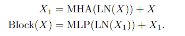
Note: The sequence of length L+1 is generated here because of spacetime resolution + class token
4. The resulting sequence after N consecutive blocks is normalized by the layer, and the output is predicted by the linear layer. It should be noted here that by default, the input of MLP is 4D.
3. Model building parameters
In Table 1 of the paper, there are parameters for three models (Base/Large/Huge). In addition to the Patch Size of 16x16 in the source code, there are also 32x32.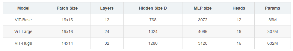
in:
Layers is the number L of repeated stacking of the Encoder Block in the Transformer Encoder. Hidden
Size corresponds to the dim (the length of the sequence vector) of each token after passing through the Embedding layer (Patch Embedding + Class Embedding + Position Embedding) 4 times) Heads represents the number of heads of Multi-Head Attention in Transformer.
4. Results analysis
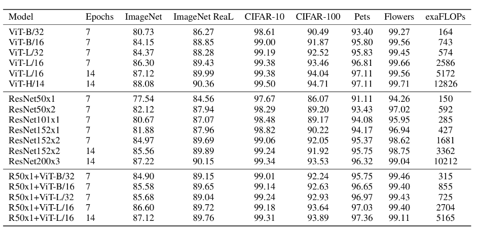
The above table is used by the paper to compare the effects of ViT, Resnet (as just mentioned, the convolutional layer and Norm layer used have been modified) and the Hybrid model. From the comparison, it can be concluded that:
1. Hybrid is better than ViT when there are fewer training epochs -> Epoch selects Hybrid
2. When the epoch increases, ViT is better than Hybrid -> Epoch general election ViT