written in front
The reference is https://zh.d2l.ai/index.html
1. Purpose and requirements of large-scale operation design
(1) Use the learned clustering algorithm to complete a simple image segmentation system.
(2) Program and use relevant software to complete large-scale homework tests and obtain experimental results.
(3) Draw experimental conclusions through the analysis of experimental results, cultivate students' innovative thinking and ability to write experimental reports, as well as the preliminary ability to deal with general engineering design technical problems and a scientific attitude of seeking truth from facts.
(4) Take advantage of the advantages of more intuitive, convenient and easy-to-operate experiments to improve students' interest in learning, let students design and implement experiments independently, and bring out their potential enthusiasm and creativity.
(5) Through the training of experiments, students can further master the image classification problem based on convolutional neural network, and further understand the significance of learning machine learning knowledge.
2. Major job design content
Big homework 1: Handwritten digit recognition system.
This project requires the selection of machine learning algorithms to design and implement a handwritten digit recognition system. Handwritten digit recognition has important applications in daily life, such as remittance slips, bank check processing, and mail sorting. Handwritten digit recognition usually requires high precision. Although there are only 10 categories, each handwriting is different, so it is difficult to achieve accurate recognition. The specific requirements of the project are as follows:
(1) Use the MNIST handwritten digit data set to perform handwritten digit recognition (refer to textbook P186, example 6.2).
(2) Select an appropriate machine learning algorithm for handwritten digit recognition and train a classification model, requiring the recognition accuracy to be as high as possible.
(3) Write a simple user interface that can load pictures of handwritten numbers and call algorithms to recognize numbers.
3. Program development and operating environment
Graphics card: NVIDIA graphics card, CUDA 11.7.
System and environment: Windows11 operating system, base virtual environment of Anaconda3.
IDE: Pycharm Community integrated development environment, Jupyter Notebook
deep learning framework: PyTorch deep learning framework, based on GPU version.
Graphical interface framework: PyQt5
4. Design text
(Including analysis and design ideas, flow charts of each module, pseudo-code of main algorithms, etc. If there is any improvement or expansion, please focus on one section for explanation)
4.1 Analysis and Design Ideas and Flowchart
The experimental task is to use the MNIST handwritten data set for handwritten digit recognition. Using traditional neural network models such as multi-layer perceptrons cannot solve such problems well, because this model directly reads the original pixels of the image and classifies them based on the original pixels of the image. However, the extraction of image features also requires artificially designed functions for extraction. Therefore, the convolutional neural network model can perform automatic feature extraction on images very well.
This big assignment uses the classic AlexNet convolutional neural network model. The AlexNet convolutional neural network model has the following overall structure:
it contains 8 layers of transformation, including 5 layers of convolution and 2 layers of fully connected hidden layers, and 1 fully connected output layer. Among them, the convolution window shape of the first layer is 11 11, which can support inputting larger images. The second-layer convolution window shape is reduced to 5 5, and the subsequent 3-layer convolution uses a 3 3 window. After the first, second, and fifth convolutional layers , maximum pooling with a convolution window size of 3 3 and a stride of 2 is used . The number of convolution channels is 10 times larger than that of LeNet. After the last convolution and pooling layer, there are two fully connected layers with an output of 4096, and finally output the result.
1. Introduce methods such as image augmentation, flipping, and cropping to further create and expand the dataset from the original dataset.
The flow chart of AlexNet is as follows:

In this experiment, because the MNIST dataset is running, the last fully connected layer has only 10 nodes instead of 1000 in the flow chart.
In order to display the graphical interface, a front-end graphical interface is also set up using the PyQt framework.
After training the data set, write the model to the hard disk file and save it for calling and reading by the front-end graphical interface.
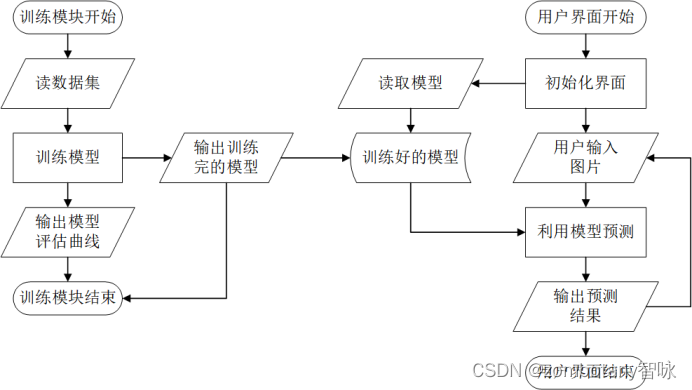
Therefore, during the initialization process of the front-end graphical interface, the trained model is pre-loaded. The user can read in the handwritten digital picture that needs to be recognized from the file, and the front-end graphical interface will automatically give the recognition result of the handwritten digital picture according to the loaded model. Therefore, the interaction logic of each module in this experiment is shown in the figure below.
4.2 Main algorithm code
training model
import numpy as np  # numpy数组库
import math  # 数学运算库
import matplotlib.pyplot as plt  # 画图库
import torch  # torch基础库
import torchvision.datasets as dataset  # 公开数据集的下载和管理
import torchvision.transforms as transforms  # 公开数据集的预处理库,格式转换
import torchvision.utils as utils
import torch.utils.data as data_utils  # 对数据集进行分批加载的工具集
from torch.utils import data
from d2l import torch as d2l
d2l.use_svg_display()
from torch import nn
net = nn.Sequential(
    # 这里,我们使用一个11*11的更大窗口来捕捉对象。
    # 同时,步幅为4,以减少输出的高度和宽度。
    # 另外,输出通道的数目远大于LeNet
    nn.Conv2d(1, 96, kernel_size=11, stride=4, padding=1), nn.ReLU(),
    nn.MaxPool2d(kernel_size=3, stride=2),
    # 减小卷积窗口,使用填充为2来使得输入与输出的高和宽一致,且增大输出通道数
    nn.Conv2d(96, 256, kernel_size=5, padding=2), nn.ReLU(),
    nn.MaxPool2d(kernel_size=3, stride=2),
    # 使用三个连续的卷积层和较小的卷积窗口。
    # 除了最后的卷积层,输出通道的数量进一步增加。
    # 在前两个卷积层之后,汇聚层不用于减少输入的高度和宽度
    nn.Conv2d(256, 384, kernel_size=3, padding=1), nn.ReLU(),
    nn.Conv2d(384, 384, kernel_size=3, padding=1), nn.ReLU(),
    nn.Conv2d(384, 256, kernel_size=3, padding=1), nn.ReLU(),
    nn.MaxPool2d(kernel_size=3, stride=2),
    nn.Flatten(),
    # 这里,全连接层的输出数量是LeNet中的好几倍。使用dropout层来减轻过拟合
    nn.Linear(6400, 4096), nn.ReLU(),
    nn.Dropout(p=0.5),
    nn.Linear(4096, 4096), nn.ReLU(),
    nn.Dropout(p=0.5),
    # 最后是输出层。由于这里使用MNIST,所以用类别数为10,而非论文中的1000
    nn.Linear(4096, 10))
X = torch.randn(1, 1, 224, 224)#随机初值
for layer in net:#用随机权重参数初始化CNN
    X=layer(X)
    print(layer.__class__.__name__,'output shape:\t',X.shape)
def load_data_mnist(batch_size, resize=None):#读取、加载MNIST数据集,并batch
    trans = [transforms.ToTensor()]
    if resize:
        trans.insert(0, transforms.Resize(resize))
    trans = transforms.Compose(trans)
    mnist_train = dataset.MNIST(
        root="../data", train=True, transform=trans, download=True)
    mnist_test = dataset.MNIST(
        root="../data", train=False, transform=trans, download=True)
    return (data.DataLoader(mnist_train, batch_size, shuffle=True,
                            num_workers=4),
            data.DataLoader(mnist_test, batch_size, shuffle=False,
                            num_workers=4))
batch_size = 128
train_iter, test_iter = load_data_mnist(batch_size=batch_size,resize=224)
for i, (X, y) in enumerate(train_iter):
    device = torch.device("cuda" if torch.cuda.is_available() else "cpu")
    X, y = X.to(device), y.to(device)
    print("X:",X.shape)
    print("y:",y.shape)
def evaluate_accuracy_gpu(net, data_iter, device=None): #@save
    """使用GPU计算模型在数据集上的精度"""
    if isinstance(net, nn.Module):
        net.eval()  # 设置为评估模式
        if not device:
            device = next(iter(net.parameters())).device
    # 正确预测的数量,总预测的数量
    metric = d2l.Accumulator(2)
    with torch.no_grad():
        for X, y in data_iter:
            if isinstance(X, list):
                # BERT微调所需的
                X = [x.to(device) for x in X]
            else:
                X = X.to(device)
            y = y.to(device)
            metric.add(d2l.accuracy(net(X), y), y.numel())
    return metric[0] / metric[1]
def train_ch6(net, train_iter, test_iter, num_epochs, lr, device):
    """用GPU训练模型(在第六章定义)"""
    def init_weights(m):
        if type(m) == nn.Linear or type(m) == nn.Conv2d:
            nn.init.xavier_uniform_(m.weight)
    net.apply(init_weights)
    print('training on', device)
    net.to(device)
    optimizer = torch.optim.SGD(net.parameters(), lr=lr)
    loss = nn.CrossEntropyLoss()
    animator = d2l.Animator(xlabel='epoch', xlim=[1, num_epochs],
                            legend=['train loss', 'train acc', 'test acc'])
    timer, num_batches = d2l.Timer(), len(train_iter)
    for epoch in range(num_epochs):
        # 训练损失之和,训练准确率之和,样本数
        metric = d2l.Accumulator(3)
        net.train()
        for i, (X, y) in enumerate(train_iter):
            timer.start()
            optimizer.zero_grad()
            X, y = X.to(device), y.to(device)
            y_hat = net(X)
            l = loss(y_hat, y)
            l.backward()
            optimizer.step()
            with torch.no_grad():
                metric.add(l * X.shape[0], d2l.accuracy(y_hat, y), X.shape[0])
            timer.stop()
            train_l = metric[0] / metric[2]
            train_acc = metric[1] / metric[2]
            if (i + 1) % (num_batches // 5) == 0 or i == num_batches - 1:
                animator.add(epoch + (i + 1) / num_batches,
                             (train_l, train_acc, None))
        test_acc = evaluate_accuracy_gpu(net, test_iter)
        animator.add(epoch + 1, (None, None, test_acc))
        animator.show()
    print(f'loss {

      train_l:.3f}, train acc {

      train_acc:.3f}, '
          f'test acc {

      test_acc:.3f}')
    print(f'{

      metric[2] * num_epochs / timer.sum():.1f} examples/sec '
          f'on {

      str(device)}')

lr, num_epochs = 0.01, 10
train_ch6(net, train_iter, test_iter, num_epochs, lr, d2l.try_gpu())

torch.save(net, "cnn.pt")
User Interface
from PIL import Image, ImageDraw, ImageFont
from PyQt5.QtWidgets import (QMainWindow, QMenuBar, QToolBar, QTextEdit, QAction, QApplication,
                             qApp, QMessageBox, QFileDialog, QLabel, QHBoxLayout, QGroupBox,
                             QComboBox, QGridLayout, QLineEdit, QSlider, QPushButton)
from PyQt5.QtGui import *
from PyQt5.QtGui import QPalette, QImage, QPixmap, QBrush
from PyQt5.QtCore import *
import sys
import cv2 as cv
import cv2
import numpy as np
import time
from pylab import *
import os
from torchvision import transforms
from PIL import Image
import torch
import numpy as np

class Window(QMainWindow):
    path = ' '
    change_path = "change.png"#被处理过的图像的路径
    IMG1 = ' '
    IMG2 = 'null'

    def __init__(self):
        super(Window, self).__init__()
        # 界面初始化

        self.createMenu()#创建左上角菜单栏
        self.cwd = os.getcwd()#当前工作目录
        self.image_show()
        self.label1 = QLabel(self)
        self.initUI()

    # 菜单栏
    def createMenu(self):
        # menubar = QMenuBar(self)
        menubar = self.menuBar()
        menu1 = menubar.addMenu("文件")
        menu1.addAction("打开")
        menu1.triggered[QAction].connect(self.menu1_process)

    #展示大图片
    def image_show(self):
        self.lbl = QLabel(self)
        self.lbl.setPixmap(QPixmap('source.png'))
        self.lbl.setAlignment(Qt.AlignCenter)  # 图像显示区,居中
        self.lbl.setGeometry(35, 35, 800, 700)
        self.lbl.setStyleSheet("border: 2px solid black")

    def initUI(self):
        self.setGeometry(50, 50, 900, 800)
        self.setWindowTitle('mnist识别系统')
        palette = QPalette()
        palette.setColor(self.backgroundRole(), QColor(255, 255, 255))
        self.setPalette(palette)

        self.label1.setText("TextLabel")
        self.label1.move(100,730)
        self.show()
    # 菜单1处理
    def menu1_process(self, q):
        self.path = QFileDialog.getOpenFileName(self, '打开文件', self.cwd,
                                                "All Files (*);;(*.bmp);;(*.tif);;(*.png);;(*.jpg)")
        self.image = cv.imread(self.path[0])
        self.lbl.setPixmap(QPixmap(self.path[0]))
        cv2.imwrite(self.change_path, self.image)
        transforms1 = transforms.Compose([
            transforms.ToTensor()
        ])
        self.label1.setText("识别中")
        img = Image.open(self.change_path)
        img = img.convert("L")
        img = img.resize((224, 224))
        tensor = transforms1(img)
        print(tensor.shape)
        tensor = tensor.type(torch.FloatTensor)
        device = torch.device("cuda" if torch.cuda.is_available() else "cpu")
        tensor = tensor.to(device)
        tensor = tensor.reshape((1, 1, 224, 224))
        print(tensor.shape)
        y = net(tensor)
        print(y)
        print(torch.argmax(y))
        self.label1.setText(str(int(torch.argmax(y))))
if __name__ == '__main__':
    net = torch.load('cnn.pt')
    app = QApplication(sys.argv)
    ex = Window()
    ex.show()
    sys.exit(app.exec_())
4.3 Improvement and expansion
1. Reconfigured the environment and installed the GPU-based version of Pytorch. Compared with the CPU version, the GPU can support faster convolution operations. At the same time, larger video memory can also support batch processing of more data batches, which is conducive to the stability of training and prevents "gradient disappearance". In the CPU version, if the batch size is too large, problems such as memory explosion may occur.
2. AlexNet replaced the sigmoid activation function with a simpler ReLU activation function. The calculation of ReLU is simpler, making the model easier to train, and will not cause "gradient disappearance" and other situations that make the model unable to be trained effectively.
3. In order to prevent overfitting, a certain probability of dropout is also introduced to control the model complexity of the fully connected layer.
5. Experimental results and analysis
(Running results and detailed analysis in different situations)
The following is the output of the python console
D:\ProgramData\Anaconda3\python.exe F:/mnist/mlhw3.py
Conv2d output shape: torch.Size([1, 96, 54, 54])
ReLU output shape: torch.Size([1, 96, 54, 54])
MaxPool2d output shape: torch.Size([1, 96, 26, 26])
Conv2d output shape: torch.Size([1, 256, 26, 26])
ReLU output shape: torch.Size([1, 256, 26, 26])
MaxPool2d output shape: torch.Size([1, 256, 12, 12])
Conv2d output shape: torch.Size([1, 384, 12, 12])
ReLU output shape: torch.Size([1, 384, 12, 12])
Conv2d output shape: torch.Size([1, 384, 12, 12])
ReLU output shape: torch.Size([1, 384, 12, 12])
Conv2d output shape: torch.Size([1, 256, 12, 12])
ReLU output shape: torch.Size([1, 256, 12, 12])
MaxPool2d output shape: torch.Size([1, 256, 5, 5])
Flatten output shape: torch.Size([1, 6400])
Linear output shape: torch.Size([1, 4096])
ReLU output shape: torch.Size([1, 4096])
Dropout output shape: torch.Size([1, 4096])
Linear output shape: torch.Size([1, 4096])
ReLU output shape: torch.Size([1, 4096])
Dropout output shape: torch.Size([1, 4096])
Linear output shape: torch.Size([1, 10])
training on cuda:0
<Figure size 350x250 with 1 Axes>
<Figure size 350x250 with 1 Axes>
<Figure size 350x250 with 1 Axes>
<Figure size 350x250 with 1 Axes>
<Figure size 350x250 with 1 Axes>
<Figure size 1920x951 with 1 Axes>
<Figure size 1920x951 with 1 Axes>
<Figure size 1920x951 with 1 Axes>
<Figure size 1920x951 with 1 Axes>
<Figure size 1920x951 with 1 Axes>
<Figure size 1920x951 with 1 Axes>
<Figure size 1920x951 with 1 Axes>
<Figure size 1920x951 with 1 Axes>
<Figure size 1920x951 with 1 Axes>
<Figure size 1920x951 with 1 Axes>
<Figure size 1920x951 with 1 Axes>
<Figure size 1920x951 with 1 Axes>
<Figure size 1920x951 with 1 Axes>
<Figure size 1920x951 with 1 Axes>
<Figure size 1920x951 with 1 Axes>
<Figure size 1920x951 with 1 Axes>
<Figure size 1920x951 with 1 Axes>
<Figure size 1920x951 with 1 Axes>
<Figure size 1920x951 with 1 Axes>
<Figure size 1920x951 with 1 Axes>
<Figure size 1920x951 with 1 Axes>
<Figure size 1920x951 with 1 Axes>
<Figure size 1920x951 with 1 Axes>
<Figure size 1920x951 with 1 Axes>
<Figure size 1920x951 with 1 Axes>
<Figure size 1920x951 with 1 Axes>
<Figure size 1920x951 with 1 Axes>
<Figure size 1920x951 with 1 Axes>
<Figure size 1920x951 with 1 Axes>
<Figure size 1920x951 with 1 Axes>
<Figure size 1920x951 with 1 Axes>
<Figure size 1920x951 with 1 Axes>
<Figure size 1920x951 with 1 Axes>
<Figure size 1920x951 with 1 Axes>
<Figure size 1920x951 with 1 Axes>
<Figure size 1920x951 with 1 Axes>
<Figure size 1920x951 with 1 Axes>
<Figure size 1920x951 with 1 Axes>
<Figure size 1920x951 with 1 Axes>
<Figure size 1920x951 with 1 Axes>
<Figure size 1920x951 with 1 Axes>
<Figure size 1920x951 with 1 Axes>
<Figure size 1920x951 with 1 Axes>
<Figure size 1920x951 with 1 Axes>
<Figure size 1920x951 with 1 Axes>
<Figure size 1920x951 with 1 Axes>
<Figure size 1920x951 with 1 Axes>
<Figure size 1920x951 with 1 Axes>
<Figure size 1920x951 with 1 Axes>
<Figure size 1920x951 with 1 Axes>
<Figure size 1920x951 with 1 Axes>
<Figure size 1920x951 with 1 Axes>
<Figure size 1920x951 with 1 Axes>
<Figure size 1920x951 with 1 Axes>
<Figure size 1920x951 with 1 Axes>
<Figure size 1920x951 with 1 Axes>
<Figure size 1920x951 with 1 Axes>
<Figure size 1920x951 with 1 Axes>
<Figure size 1920x951 with 1 Axes>
<Figure size 1920x951 with 1 Axes>
<Figure size 1920x951 with 1 Axes>
<Figure size 1920x951 with 1 Axes>
<Figure size 1920x951 with 1 Axes>
<Figure size 1920x951 with 1 Axes>
<Figure size 1920x951 with 1 Axes>
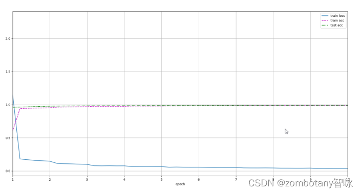
loss 0.039, train acc 0.988, test acc 0.991
624.4 examples/sec on cuda:0
It can be seen that the model is correctly established, and the process of iteration, update and training is carried out correctly. After the training is completed, the loss function is 0.039, the accuracy rate of the training set is 0.988, and the accuracy rate of the test set is 0.991. On cuda, 624 training data are run every second.
The change curves of training set accuracy, test set accuracy, and loss function are as follows. It can be seen that the recognition accuracy is very high.
This is a graphical user interface

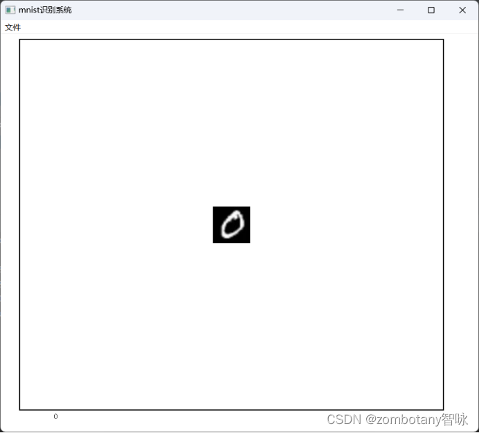
that can read files,
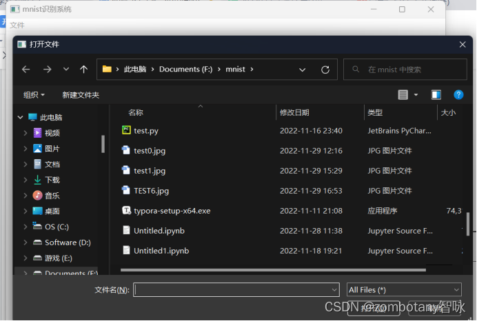
read pictures of the number "0" and identify them correctly. This picture is a picture of real handwriting and inverse color processing, not from the training set.
The console output is as follows:
torch.Size([1, 224, 224])
torch.Size([1, 1, 224, 224])
tensor([[16.5969, -2.6974,  1.0315, -4.3109, -2.4112, -2.2494,  2.9837, -2.5753,
         -1.0474,  0.4374]], device='cuda:0', grad_fn=<AddmmBackward0>)
tensor(0, device='cuda:0')
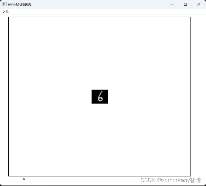
The user interface is as follows:
read the number "6" and recognize it correctly. This picture is a picture of real handwriting and inverse color processing, not from the training set.
The console output is as follows:
torch.Size([1, 224, 224])
torch.Size([1, 1, 224, 224])
tensor([[-3.4247, -0.9304, -0.6991, -1.0964,  0.0769,  2.2364, 11.2306, -6.2827,
          6.0278, -7.4283]], device='cuda:0', grad_fn=<AddmmBackward0>)
tensor(6, device='cuda:0')
The user interface is as follows:
6. Summary and further improvement ideas
In this experiment, the classic MNIST dataset was trained using the classic AlexNet convolutional neural network. After completing the tasks of model building and training, the recognition accuracy is high enough, and a simple user interface was written, and tested with real handwritten pictures. It can be seen that the model is also applicable to real scenes, not just for loading Come out and split out the test set.
For further improvement, methods such as image augmentation, flipping, cropping, and color changes can be introduced to further expand the production data set for training and testing. It is possible to use 3-channel color maps of RGB colors instead of just using single-channel binarized images for training.
7. References
[1] Zhou Zhihua. Machine Learning [M]. First Edition in January 2016. Beijing: Tsinghua University Press, 2016. [
2] Zhao Weidong, Dong Liang. Machine Learning [M]. First Edition in August 2018. Beijing: People's Posts and Telecommunications Press, 2018.
[3] Li Hang. Statistical Learning Methods [M]. 2nd Edition, May 2019. Beijing: Tsinghua University Press, 2019. [4
] Aston Zhang ), Li Mu (Mu Li), [US] Zachary C. Lipton (Zachary C. Lipton), et al. Hands-on Deep Learning [M]. 1st Edition, June 2019. Beijing: People's Posts and Telecommunications Press , 2019.
[5] [US] Ian Goodfellow [Add] Yoshua Bengio [Add] Aaron Courville. Deep Learning [M]. 1st Edition in August 2017. Beijing: People's Posts and Telecommunications Press, 2017.