Image map
The my_Kalman.ipynb and ppt inside are enough, the others are original data and auxiliary functions
Link: https://pan.baidu.com/s/1J1nA–oqoj8OvgbrA3LfbQ?pwd=1264
Extraction code: 1264
import numpy as np
import matplotlib.pyplot as plt
from matplotlib.animation import FuncAnimation
# 定义卡尔曼滤波器类
class KalmanFilter:
    def __init__(self, dt, sigma_a, sigma_z):
        self.dt = dt  # 时间步长
        self.sigma_a = sigma_a  # 过程噪声的标准差
        self.sigma_z = sigma_z  # 观测噪声的标准差
        self.A = np.array([[1, 0, dt, 0],
                           [0, 1, 0, dt],
                           [0, 0, 1, 0],
                           [0, 0, 0, 1]])  # 状态转移矩阵
        self.Q = np.array([[dt**4/4, 0, dt**3/2, 0],
                           [0, dt**4/4, 0, dt**3/2],
                           [dt**3/2, 0, dt**2, 0],
                           [0, dt**3/2, 0, dt**2]]) * sigma_a**2  # 过程噪声协方差矩阵
        self.H = np.array([[1, 0, 0, 0],
                           [0, 1, 0, 0]])  # 观测矩阵
        self.R = np.array([[sigma_z**2, 0],
                           [0, sigma_z**2]])  # 观测噪声协方差矩阵
        self.mu = np.zeros((4, 1))  # 状态向量
        self.sigma = np.eye(4)  # 状态协方差矩阵

    # 预测状态和协方差
    def predict(self):
        self.mu = self.A @ self.mu
        self.sigma = self.A @ self.sigma @ self.A.T + self.Q

    # 更新状态和协方差
    def update(self, z):
        K = self.sigma @ self.H.T @ np.linalg.inv(self.H @ self.sigma @ self.H.T + self.R)
        self.mu = self.mu + K @ (z - self.H @ self.mu)
        self.sigma = (np.eye(4) - K @ self.H) @ self.sigma

    # 获取当前状态向量
    def get_state(self):
        return self.mu.flatten()[:2]

# 初始化参数
dt = 0.1  # 时间步长
sigma_a = 0.5  # 过程噪声的标准差
sigma_z = 1  # 观测噪声的标准差
u = np.array([1, 0.5, 0, 0])  # 物体的速度和加速度
x_real = np.array([0, 0])  # 物体的真实位置
kf = KalmanFilter(dt, sigma_a, sigma_z)  # 初始化卡尔曼滤波器

# 绘制预测结果的动态可视化
fig, ax = plt.subplots()
xdata_real, ydata_real = [], []
xdata_pred, ydata_pred = [], []
line_real, = ax.plot([], [], 'o', color='blue')
line_pred, = ax.plot([], [], '-', color='red')

def init():
    ax.set_xlim(-10, 10)
    ax.set_ylim(-10, 10)
    return line_real, line_pred

def update(frame):
    global x_real, u, kf
    # 更新物体的真实位置
    x_real = x_real + u[:2] * dt
    # 产生观测值
    z = x_real + np.random.randn(2) * sigma_z
    # 进行预测和更新
    kf.predict()
    kf.update(z)
    # 绘制真实位置和预测位置
    xdata_real.append(x_real[0])
    ydata_real.append(x_real[1])
    line_real.set_data(xdata_real, ydata_real)
    x_pred, y_pred = kf.get_state()
    xdata_pred.append(x_pred)
    ydata_pred.append(y_pred)
    line_pred.set_data(xdata_pred, ydata_pred)
    return line_real, line_pred

ani = FuncAnimation(fig, update, frames=range(100), init_func=init, blit=True)

# 保存动态图为gif文件
ani.save('kalman_filter_prediction.gif', writer='pillow')
We define a KalmanFilter class to implement the Kalman filter. In the update function, we first update the real position of the object, then generate observations, then use the Kalman filter to predict and update, and plot the real and predicted positions on the image. At the same time, we use the FuncAnimation function to dynamically visualize the prediction results, and use the ani.save function to save the dynamic graph as a gif file.
After the code is executed, a file named kalman_filter_prediction.gif will be generated in the current working directory, which contains the drawn dynamic graph. You can open it with any image viewer that supports gif format.
A Kalman filter is an algorithm that uses a sequence of measurements observed over time to estimate the state of a system. It is widely used in many different fields of engineering and science, including control systems, signal processing, and robotics.
At a high level, a Kalman filter works by combining two streams of information: predictions about the current state of the system and measurements of the actual state of the system. The filter uses these two streams of information to iteratively update its estimate of the state of the system and calculate the uncertainty (or covariance) of that estimate.
More specifically, the Kalman filter follows a recursive process that includes the following steps:
-
Prediction: The filter predicts the current state of the system based on previous estimates of the state and the dynamics of the system (i.e. the evolution of the state over time). This forecast is based on a state transition model, describing the evolution of the state over time, and a process noise model, which takes into account any uncertainty or error in the forecast.
-
Update: The filter incorporates new measurements of the system (i.e., observations) and updates its estimate of the state based on the difference between the predicted state and the observed state. This update is based on a measurement model that describes the relationship of the measurements to the state of the system, and a measurement noise model that accounts for any uncertainty or error in the measurements.
-
Repeat: The filter repeats these steps, using the updated state estimate as a prediction for the next time step, and incorporating new measurements to improve its estimate.
The Kalman filter aims to minimize the mean squared error between the estimated state and the true state of the system. It does this by minimizing the expected squared error between the estimated state and the true state, given available measurements and predictions, using a set of mathematical equations.
Overall, the Kalman filter is a powerful tool for estimating the state of a system in the presence of uncertainty and noise. It is widely used in many different fields and has been proven effective in a wide range of applications.

What is a Kalman filter
Kalman Filter (Kalman Filter) is an algorithm for estimating the state variables in the state space model, which can recursively calculate and update the estimated value and error covariance matrix of the state through the dynamic equations and observation equations of the system. The Kalman filter algorithm was first proposed by RE Kalman in 1960, and has been widely used in control, signal processing, aerospace, wireless communication, robotics and other fields.
The basic idea of Kalman filtering is: through the estimation of the system state and its error, combined with the observation data to update the system state, so as to improve the estimation accuracy of the system state. Specifically, the Kalman filter algorithm includes the following steps:
-
Prediction: According to the dynamic equation of the system, using the state estimation value and error covariance matrix at the previous moment, predict the state estimation value and error covariance matrix at the current moment.
-
Update: According to the observation equation, using the observed data at the current moment and the predicted state estimation value, calculate the state estimation value and the error covariance matrix at the current moment.
-
Recursion: Prediction and update are repeated to gradually approach the real system state.
The advantage of the Kalman filter algorithm is that it can estimate the system state in real time, while considering the dynamic characteristics of the system and observation noise. It can still estimate the state of the system more accurately in the case of large noise and lack of observation data. The disadvantage is that the dynamic equations and observation equations of the system need to be modeled, and there are certain requirements for the accuracy of the model and the selection of parameters.
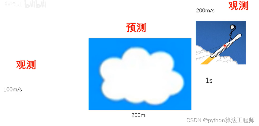
 What if the rocket is obscured?
Tracking motion, also known as motion tracking, refers to automatically or semi-automatically tracking the position and motion of a target in a video or image sequence. Tracking motion can be used in many applications such as video surveillance, autonomous driving, robot navigation, motion analysis, etc.
The target of tracking motion is usually one or more moving objects, such as people, cars, balls, etc. The process of tracking motion typically involves the following steps:
-
Object detection: Detecting the location and size of a target object in a video or image sequence.
-
Feature extraction: extract the features of the target object, such as color, texture, shape, etc.
-
Similarity measure: Calculate the similarity of the target object in adjacent frames to determine the direction and speed of the target.
-
Target tracking: Estimate the position and motion information of the target in the current frame based on the position and motion information of the target object in the previous frames.
Tracking motion is a complex task that requires the application of techniques such as computer vision and machine learning. Commonly used tracking algorithms include Kalman filter, particle filter, correlation filter, optical flow method, etc.
What is track motion?
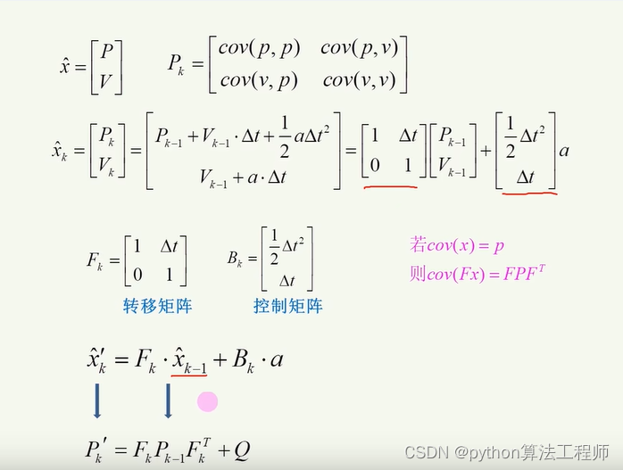
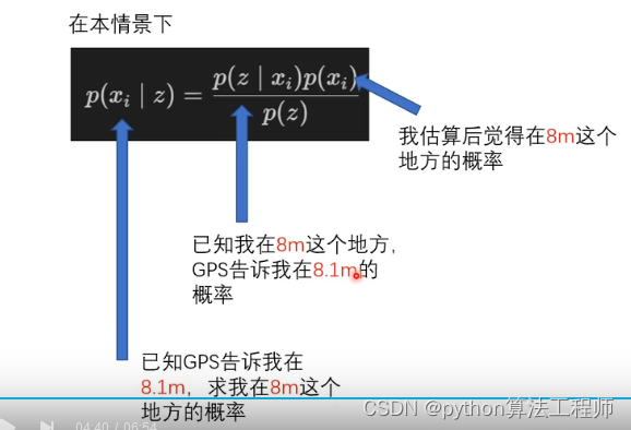
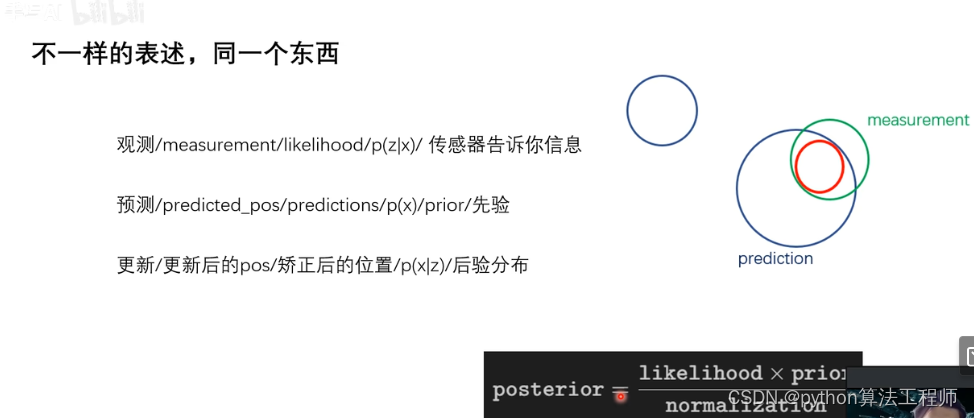
Observation
Prediction
Observation
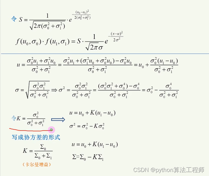
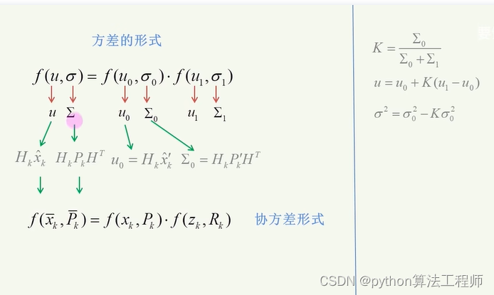
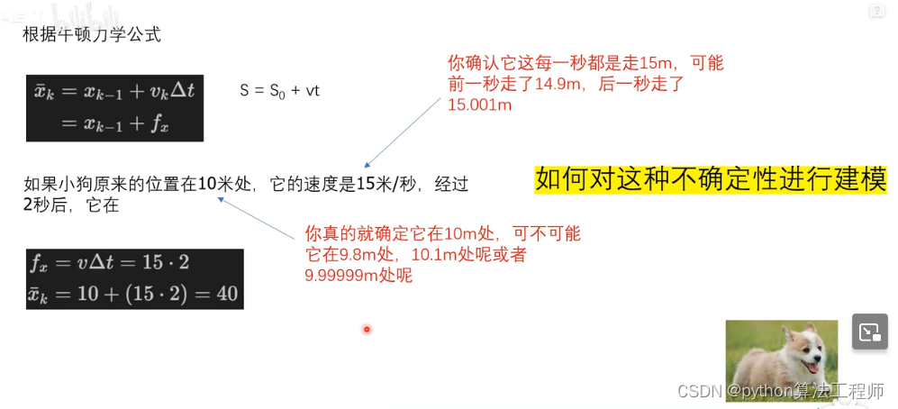
motion modeling
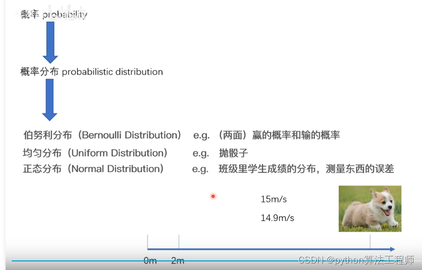
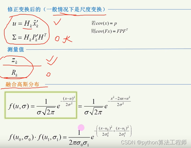
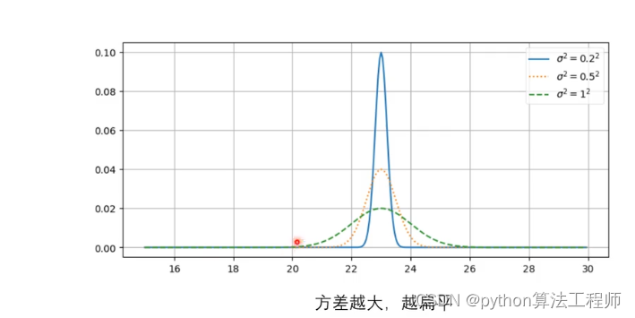
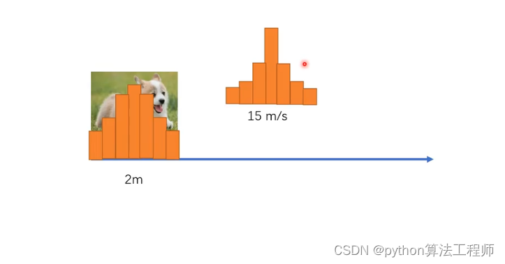 Gaussian distribution
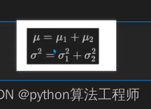
Due to the uncertainty of the dog's movement, the dog is modeled, and the Gaussian distribution is used for modeling. The Gaussian
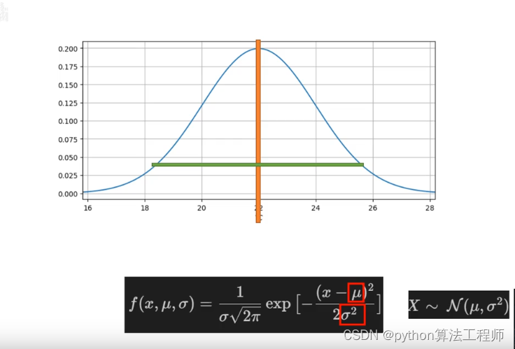 distribution is described by only two variables, the mean and the variance.
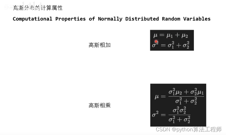
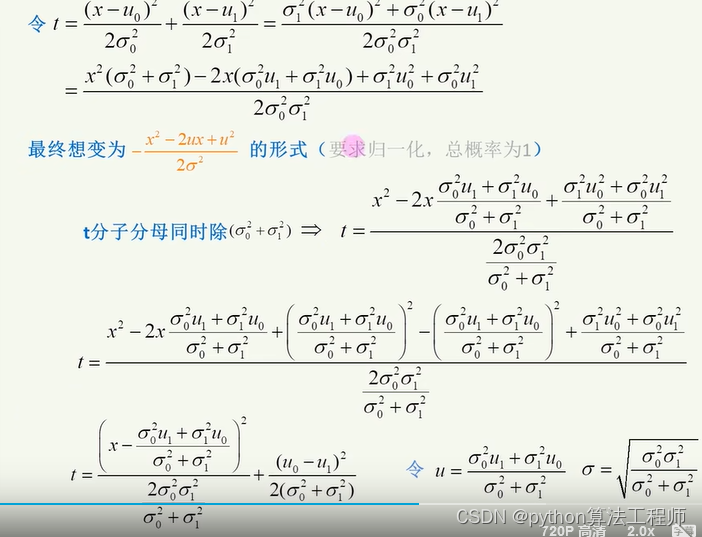
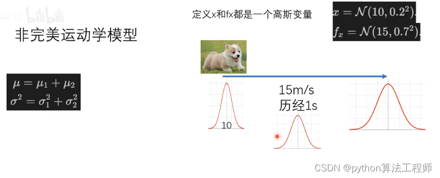
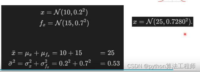
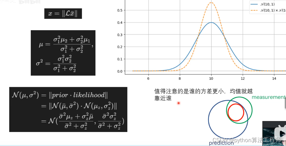
Gaussian distributions are added and multiplied and are still Gaussian. The
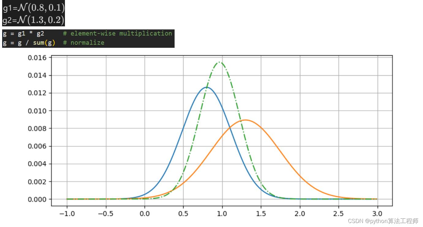
green color of the distribution The dotted line is generated by the addition of blue and yellow. The
new Gaussian distribution
mean is between the original two means. The variance becomes smaller and becomes taller and thinner.
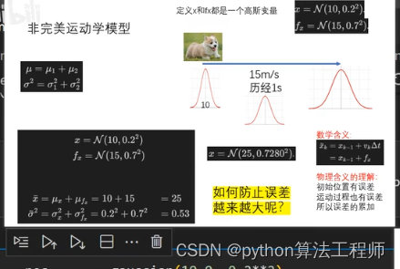
Motion prediction under Gaussian distribution
The variance of a model based on the original data
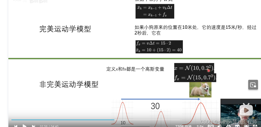 is not perfect, and the kinematic model will be larger, because its uncertainty is larger and

 the error is corrected by observation.
Optimization Algorithms: Use optimization algorithms, such as Extended Kalman Filter (EKF), Unscented Kalman Filter (UKF), etc., to optimize the position and motion of the robot or vehicle. These algorithms can reduce error accumulation and improve position and motion accuracy through joint estimation of measurements and models.
Kalman Filter is an algorithm for estimating the state of a system, which can be used to correct position and motion errors in mobile systems such as robots or vehicles. The basic principle of Kalman filtering is to estimate the true state of the system and reduce its estimation error through the fusion of the prediction of the system state and the measurement results.
The following are the general steps to correct position and motion errors using Kalman filtering:
-
Determine state variables: Determine the state variables of the system, such as the position, velocity, acceleration, etc. of the robot or vehicle.
-
Establish a state transition model: establish a state transition model to describe the change of the system state in time. For example, a kinematic model can be used to describe the motion behavior of a robot or vehicle.
-
Build an observation model: Build an observation model to describe the relationship between the system state and the measurement results. For example, sensors can be used to measure the position and motion of a robot or vehicle to build an observation model.
-
Initialization: Initialize the system state and the state of the Kalman filter. Typically, the system state is set to the initial position and velocity, and the state of the Kalman filter is set to the initial state.
-
Prediction: Using the state transition model, predict the state and covariance matrix of the system. The predicted state and covariance matrix will be used as input for the next step.
-
Measurement update: Using the observed model and measurement results, the system state and covariance matrix are updated. According to the principle of Kalman filtering, the measurement results will be used to correct the predicted state and covariance matrix.
-
Loop iteration: Repeat steps 5 and 6 until the preset condition is met or the accuracy requirement is met.
Through these steps, Kalman filtering can be used to correct the position and motion errors in the mobile system and improve its position and motion accuracy. It should be noted that the effect of Kalman filtering is affected by the accuracy and precision of the state transition model and observation model, so it needs to be adjusted and optimized according to the specific situation.
Motion prediction code for handwritten Gaussian distribution
#namedtuple
#先写一个高斯类
#导入命名元组
from collections import namedtuple
#gaussian表示一个高斯分布mean表示均值,var表示方差
gaussian = namedtuple("Gaussian",["mean","var"])
#打印出属性
gaussian.__repr__ = lambda s:f"N(mean={

      s[0]:.3f},var ={

      s[1]:.3f})"
g1 = gaussian(3.4,10.1)
g2 = gaussian(mean = 4.5, var = 0.2**2)
print(g1)
print(g2)
g1.mean,g2.var
N(mean=3.400,var =10.100)
N(mean=4.500,var =0.040)
#高斯相加
def predict(pos,movement):
#均值相加,方差相加
	return gaussian(pos.mean+movement.mean,pos.var+movement.var)
Forecast under Gaussian distribution
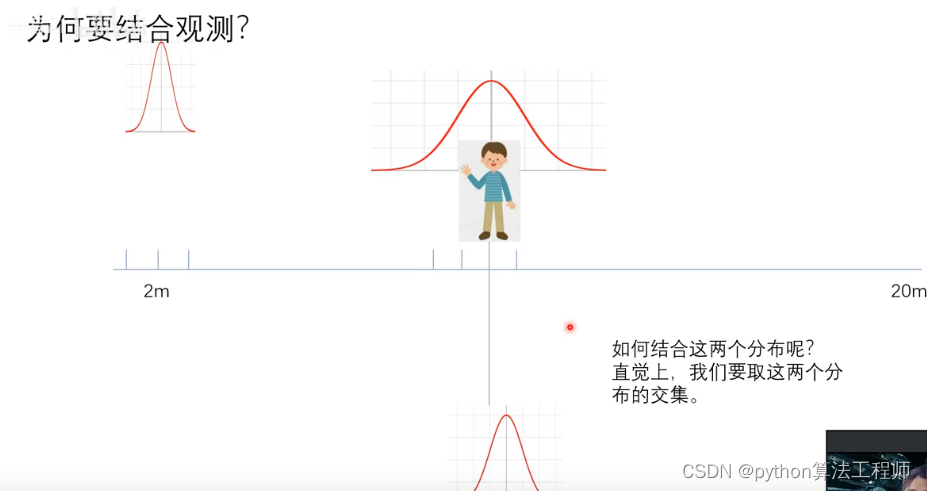
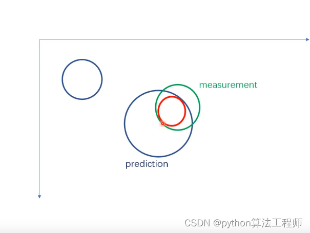 Take the intersection of two Gaussians
code demo
#高斯相乘的函数
def gaussian_multiply(g1,g2):
mean = (g1.var*g2.mean+g2.var*g1.mean)/(g1.var+g2.mean)
variance = (g1.var*g2.var)/(g1.var+g2.var)
return gaussian(mean,variance)
#更新
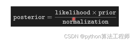
def update(likelihood,prior)
posterior = gaussian_multiply(likelihood,prior)
return posterior
predicted_pos = gaussian(10.0,0.2**2)
measured_pos = gaussian(11.0,0.1**2)
estimated_pos = update(predicted_pos,measured_pos)
print(measured_pos)
print(predicted_pos)
print(estimated_pos)
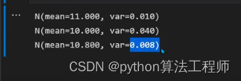 When we combine observations and predictions, we find that the variance becomes smaller
After weighted averaging of multiple data sources, it becomes more certain
Your first Kalman filter
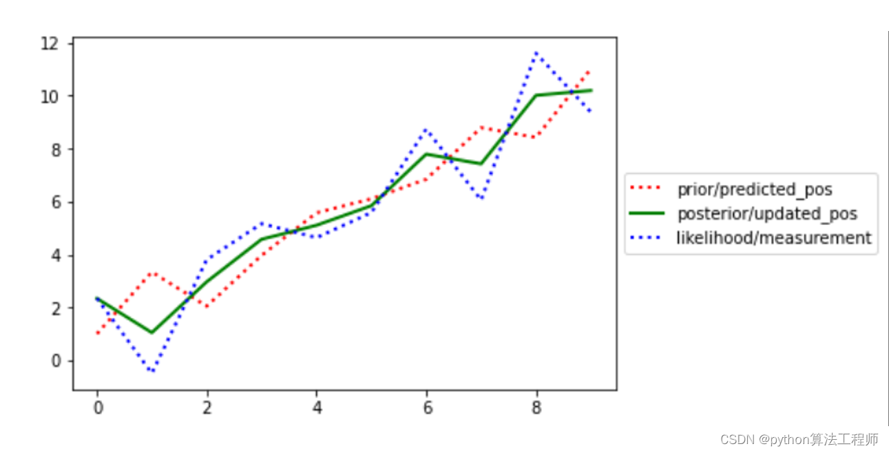 Blue and red are data sources,
green is after noise filtering
import numpy as np
from numpy.random import randn
from math import sqrt
import matplotlib.pyplot as plt
def print_result(predict,update,z,epoch):
    #predicted_pos,updated_posclear,measured_pos
    predict_template = '{:3.0f} {:7.3f} {:8.3f}'
    update_template = '\t{:.3f}\t{:7.3f}{:7.3f}'
    print(predict_template.format(epoch,predict[0],predict[1],end='\t'))
    print(update_templatre.format(z,update[0],update[1]))
def plot_result(epochs,prior_list,x_list,z_list):
    epoch_list = np.arrange(epochs)
    plt.plot(epoch_list,prior_list,linestyle = ':',color = 'r',label = "prior/predicted_pos",lw=2)
    plt.plot(epoch_list,z_list,linestyle = ":",color = 'b',label = "posterior/updated_pos",lw =2)
    plt.plot(epoch_list,z_list,linestyle=":",color = 'b',label = "likelihood.measurement",lw = 2)
    plt.legent(loc = "center left",bbox_to_anchor=(1,0.5))
#1.一些初始的状态和变量的赋值
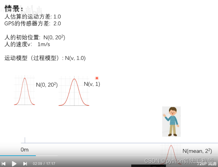
motion_var= 1.0#人的运动运动方差
sensor_var= 2.0 #GPS的运动方差
x = gaussian(0,20**2)
velocity = 1.0
dt = 1 #时间单位的最小刻度
motion_model = gaussian(velocity,motion_var)
#2.生成数据
zs = []
current_x = x.mean
for _ in range(10):#我们让小明周10s,每走1s,就看看gps进行矫正并且把这些数据存起来
#先生成我们的运动数据
v = velocity + randn()*motion_var
current_x += v*dt #将上一秒的位移加到这一秒
#生成观测数据
measurement = current_x + randn()*sensor_var#gps观测也有一定误差
zs.append(measurement)
zs
[1.7745837204798636,
 0.7238059161348066,
 2.2738223282592034,
 5.1347547337355195,
 5.692724470550488,
 5.01630210516077,
 7.273752372058138,
 10.711965916869577,
 8.341629923352198,
 10.715059361392347]