ConvNeXt principle + detailed code explanation (transparent)

ConvNeXt
Paper Name: A ConvNet for the 2020s
Paper Download Link: https://arxiv.org/abs/2201.03545
Source Code Link: https://github.com/facebookresearch/ConvNeXt
Sunflower’s Little Mung Bean Video Explanation: https://www.bilibili. com/video/BV1SS4y157fu

1 Introduction

Since ViT(Vision Transformer)it shined in the field of CV, more and more researchers began to embrace Transformerit. Looking back on the past year, most of the articles published in the field of CV are based on Transformer, such as the best paper of ICCV in 2021 Swin Transformer, and 卷积神经网络it has gradually faded out of the center of the stage. Are convolutional neural networks about to be Transformerreplaced? Maybe in the near future. In January of this year (2022), Facebook AI Researchhe and UC BerkeleyI published an article together A ConvNet for the 2020s, in which we proposed ConvNeXta pure convolutional neural network, which is very popular in 2021. Swin TransformerThrough a series of experimental comparisons, under the same FLOPs, ConvNeXtthe corresponding Compared Swin Transformerwith having faster reasoning speed and higher accuracy rate, the accuracy rate achieved on ImageNet 22Kthe above , see the figure below (original Table 12). It seems that the proposal forcibly continued the life of the convolutional neural network. After reading this article, you will find that there is "no bright spot", all the existing structures and methods are used, and there is no innovation of any structure or method. And the source code is also very streamlined, more than 100 lines of code can be built, which is not too simple. When I looked at it before , the sliding window and relative position index were not only a bit difficult to understand the principle, but the source code was also quite disappointing (but the success cannot be denied and the design is very ingenious). Why are architecture-based models now better than convolutional neural networks? The author of the paper believes that it may be that with the continuous development of technology, various new architectures and optimization strategies make the model more effective, so can using the same strategy to train the convolutional neural network achieve the same effect? With this question in mind, the authorConvNeXt-XL87.8%ConvNeXt

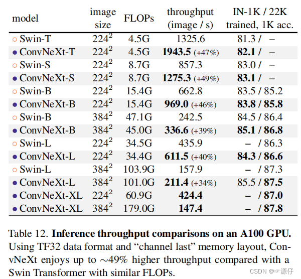
ConvNeXtConvNeXtSwin TransformerSwin TransformerSwin TransformerTransformerTransformerSwin TransformerA series of experiments were performed as a reference.

In this work, we investigate the architectural distinctions between ConvNets and Transformers and try to identify the confounding variables when comparing the network performance. Our research is intended to bridge the gap between the pre-ViT and post-ViT eras for ConvNets, as well as to test the limits of what a pure ConvNet can achieve.

2. Design plan

The author first uses the training vision Transformersstrategy to train the original ResNet50model, and finds that the effect is much better than the original, and uses this result as a benchmark for subsequent experiments baseline. Then the author lists what parts of the next experiment include:

• macro design
• ResNeXt
• inverted bottleneck
• large kerner size
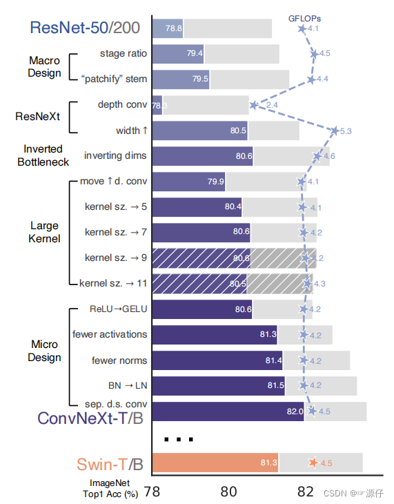
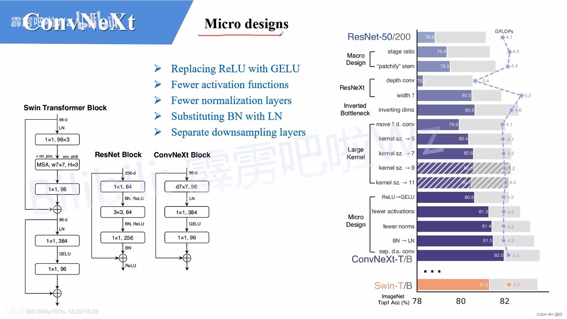
• The figure below of various layer-wise micro designs
  (Figure 2 of the original paper) shows the impact of each scheme on the final result (the accuracy of Imagenet 1K). Obviously, the final ConvNeXtaccuracy rate under the same FLOPs has exceeded Swin Transformer. Next, parse for each experiment.
  

3、Macro design

In this part, the author mainly studies two aspects:

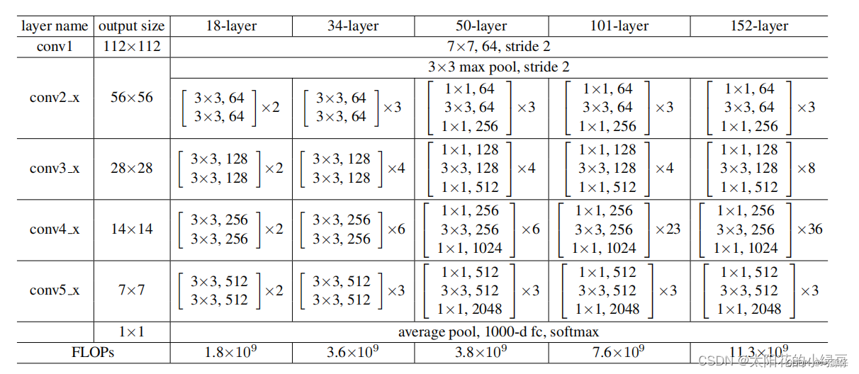
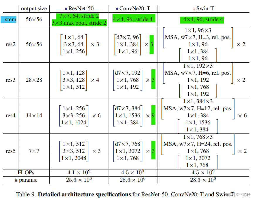
• Changing stage compute ratio , in the originalResNetnetwork, generallyconv4_x(iestage3) the number of stacked blocks is the largest. The ratio of the number of times tostack blocksResNet50inthe figure belowis about, but inthe middle, for example,the ratio is,and the ratio is. Obviously,in,stacked. So the authorrounded upthe number of stacks in, which issimilar to owning. After adjustments, the accuracy rateincreased from.stage1stage4(3, 4, 6, 3)1:1:2:1Swin TransformerSwin-T1:1:3:1Swin-L1:1:9:1Swin Transformerstage3block占比更高ResNet50(3, 4, 6, 3)(3, 3, 9, 3)Swin-TFLOPs78.8%79.4%
  
• Changing stem to "Patchify" , in the previous convolutional neural network, the general initial downsampling modulestemis generally composed of a convolutional layer with asizeof 0 and a downsampling of , and卷积核the7x7heightandwidthare downsampled 4 times. However, indown-sampledthrough a convolutional layer with a very large convolution kernel and no overlap between adjacent windows (that is,equalFor example,aconvolution layerand, which is also downsampled by 4 times. So the authorreplaced the oneinthe same one. After the replacement, the accuracy rateincreased from to, and the FLOPs also decreased a little.stride2stride2MaxPoolingTransformerstridekernel_sizeSwin Transformer4x4stridepatchifyResNetstemSwin Transformerpatchify79.4%79.5%
  

4、ResNeXt-ify

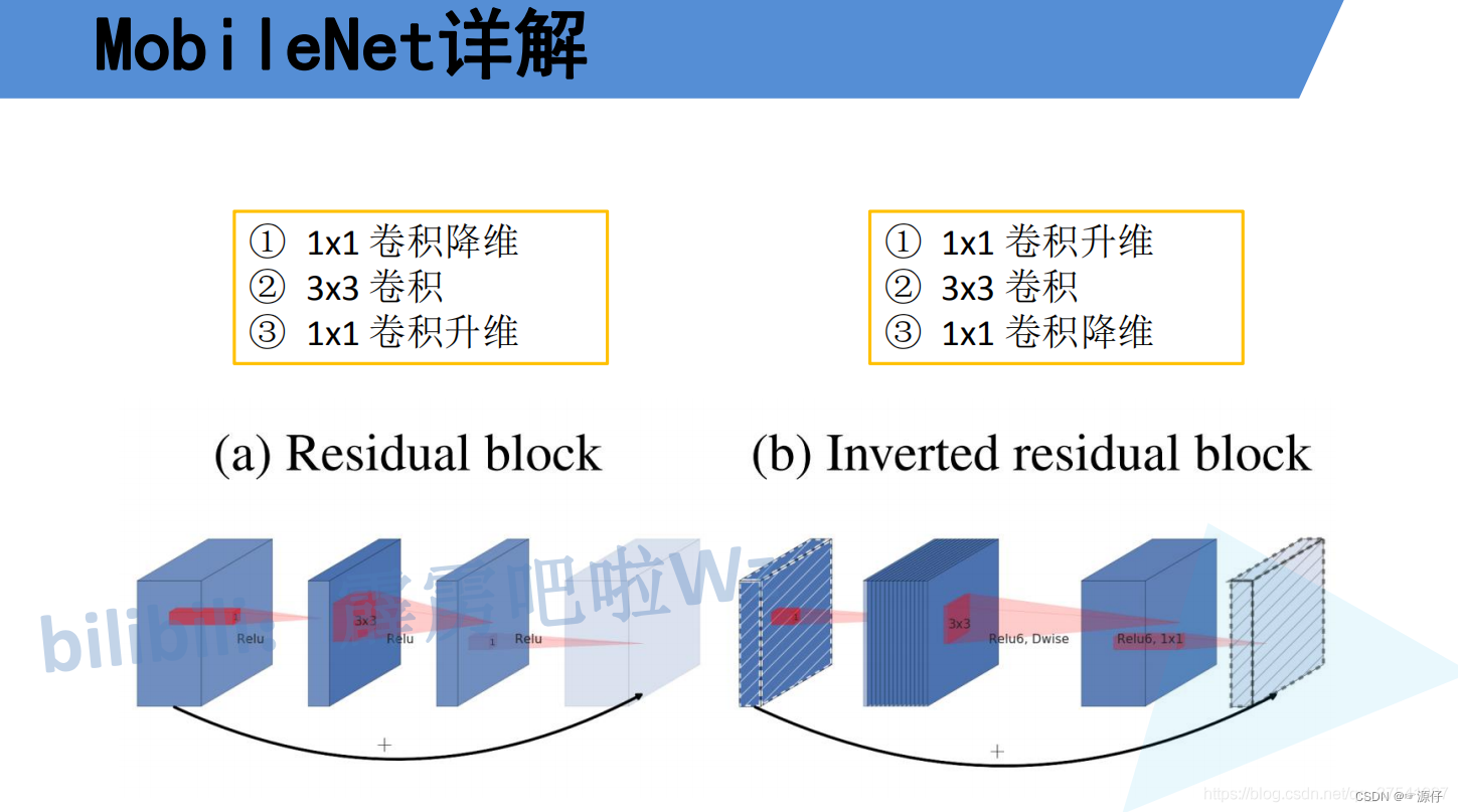
Next, the author borrowed ResNeXtthe group convolution in grouped convolution, because ResNeXtit achieves a better balance between FLOPs and accuracy than ordinary ResNet. The author adopts a more radical method depthwise convolution: that is, the number of groups is the same as the number of channels , and the detailed content can be found MobileNetin the paper.这样做的另一个原因是作者认为depthwise convolution和self-attention中的加权求和操作很相似。

We note that depthwise convolution is similar to the weighted sum operation in self-attention.

Then the author adjusted the initial 通道数from 64 to 96 and Swin Transformerkept it consistent, and the final accuracy rate was achieved 80.5%.

5、Inverted Bottleneck

The author thinks that the module Transformer blockin MLPis very similar to the module MobileNetV2in Inverted Bottleneck, that is, the two ends are thin and the middle is thick. The following picture a is the module ResNetused in the picture Bottleneck, b is MobileNetV2the used Inverted Botleneckmodule (the last 1x1 convolutional layer in picture b is wrongly drawn, it should be 384->96, and the author should correct it later if found), and c is the ConvNeXtused is Inverted Bottleneckthe module. For MLPmodule details, you can read the Vision Transformer paper, and for Inverted Bottleneckmodules, please refer to MobileNetv2 .

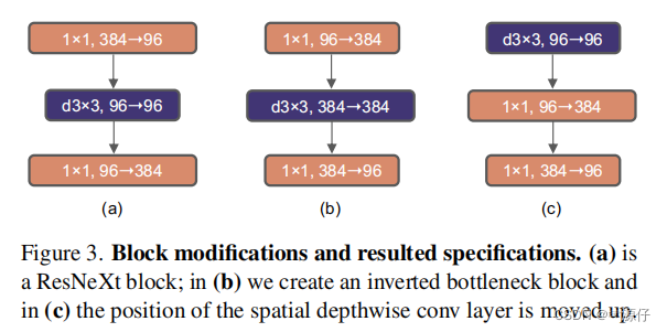
After the author adopts Inverted Bottleneckthe module, 小the accuracy rate on the better model 80.5%is improved from 1 80.6%to 2, and 大the accuracy rate on the better model 81.9%is improved from 1 to 2 82.6%.

Interestingly, this results in slightly improved performance (80.5% to 80.6%). In the ResNet-200 / Swin-B regime, this step brings even more gain (81.9% to 82.6%) also with reduced FLOPs.

6、Large Kernel Sizes

In Transformergeneral, it is done for the whole world self-attention, for example Vision Transformer. Even the windows Swin Transformerhave 7x7sizes. But now the mainstream convolutional neural network uses 3x3a large and small window, because the previous VGGpaper said that 3x3a larger window can be replaced by stacking multiple windows, and the current GPU device 3x3has done a lot of optimization for the large and small convolution kernel. , so it will be more efficient. Then the author made the following two changes:

• Moving up depthwise conv layer is to depthwise convmove the module up. It used to be 1x1 conv-> depthwise conv-> 1x1 conv, but now it becomes depthwise conv-> 1x1 conv-> 1x1 conv. The reason for doing this is because in Transformer, MSAthe module is placed MLPbefore the module, so follow the example here and depthwise convmove it up. After such a change, the accuracy rate dropped to 79.9%, and also FLOPsdecreased.
• Increasing the kernel size , and then the author changed depthwise convthe size of the convolution kernel to be the same as the Swin Transformer), of course, the author also tried other sizes, including finding that the accuracy rate reached saturation when it was taken to 7. And the accuracy rate increases from to .3x37x7（3, 5, 7, 9, 1179.9% (3×3) 80.6% (7×7)
  

7、Micro Design

Next, the author is focusing on some more subtle differences, such as activation functions and Normalization.

• Replacing ReLU with GELU , Transformerthe activation function is basically used in the middle GELU, and the most commonly used in the convolutional neural network ReLU, so the author replaced the activation function with GELU, and found that the accuracy rate did not change after the replacement.

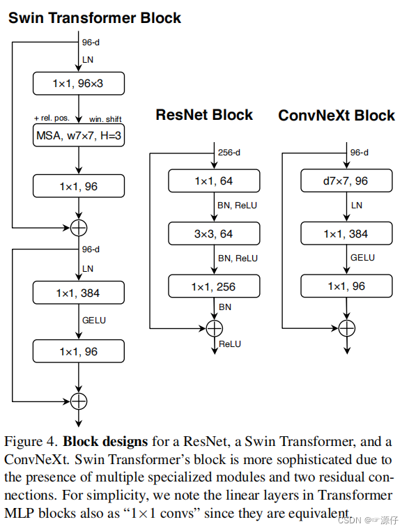
• Fewer activation functions , use fewer activation functions. In a convolutional neural network, an activation function is generally connected after each convolutional layer or full connection. However, not every module in Transformer is followed by an activation function. For example, in MLP, only the first fully connected layer is followed by a GELU activation function. Then the author also reduced the use of the activation function in the ConvNeXt Block, as shown in the figure below, after the reduction, it was found that the accuracy rate increased from 80.6% to 81.3%.
  

• Fewer normalization layer s, use less Normalization. Also in Transformer, Normalization is used less, and then the author also reduced ConvNeXt Blockthe Normalization layer in , and only kept depthwise convthe last Normalization layer. At this time, the accuracy rate has reached 81.4%and surpassed Swin-T.

• Substituting BN with LN , replace BN with LN. Batch Normalization (BN) is a very common operation in convolutional neural networks. It can speed up the convergence of the network and reduce overfitting (but it is also a big pit if it is not used well). But TransformerLayer Normalization (LN) is basically used in the Internet, because it Transformerwas originally applied in the field of NLP, and BN is not suitable for NLP-related tasks. Then the author replaced all BNs with LNs, and found that the accuracy rate was slightly improved 81.5%.

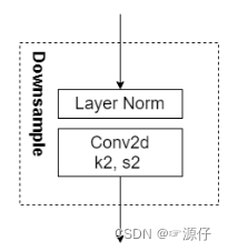
• Separate downsampling layers , a separate downsampling layer. The downsampling in ResNetthe network stage2-stage4is performed by setting the step size of the 3x3 convolutional layer on the main branch to 2, and setting the step size of the 1x1 convolutional layer on the shortcut branch to 2 for downsampling. But in Swin Transformeris through a separate Patch Mergingimplementation. Then the author ConvNextused a single downsampling layer for the network, which is composed of a Laryer Normalization plus a convolutional layer with a convolution kernel size of 2 and a step size of 2. After the change, the accuracy rate increased to 82.0%.

8、ConvNeXt variants

For ConvNeXtthe network, the author proposes T/S/B/Lfour versions, and the computational complexity is just similar to Swin Transformerthat in T/S/B/L.

We construct different ConvNeXt variants, ConvNeXt-T/S/B/L, to be of similar complexities to Swin-T/S/B/L.

The four versions are configured as follows:

• ConvNeXt-T: C = (96, 192, 384, 768), B = (3, 3, 9, 3)
• ConvNeXt-S: C = (96, 192, 384, 768), B = (3, 3, 27, 3)
• ConvNeXt-B: C = (128, 256, 512, 1024), B = (3, 3, 27, 3)
• ConvNeXt-L: C = (192, 384, 768, 1536), B = (3, 3, 27, 3)
• ConvNeXt-XL: C = (256, 512, 1024, 2048), B = (3, 3, 27, 3) where C represents the number of input channels in
  4 , and B represents the number of times each block is repeated.stagestage

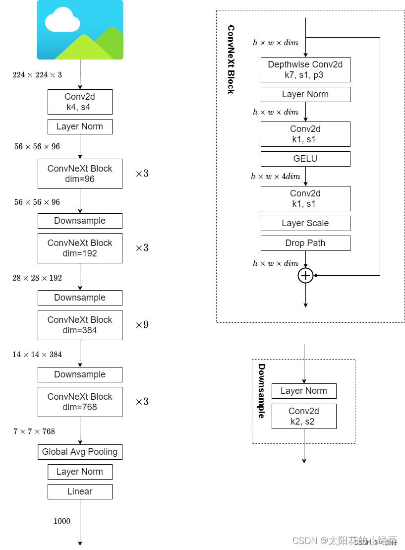
9. ConvNeXt-T structure diagram

code part

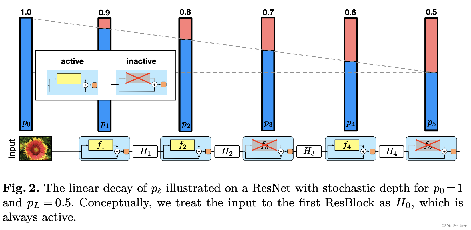
1、Stochastic Depth

Code download address: pytorch_classification/ConvNeXt
Paper address: Deep Networks with Stochastic Depth
For the convenience of implementation, the source code is not used here.
 DropPath/drop_path is a regularization method, and its effect is to randomly "delete" the multi-branch structure in the deep learning model. The implementation in python is as follows:

def drop_path(x, drop_prob: float = 0., training: bool = False):
    """Drop paths (Stochastic Depth) per sample (when applied in main path of residual blocks).

    This is the same as the DropConnect impl I created for EfficientNet, etc networks, however,
    the original name is misleading as 'Drop Connect' is a different form of dropout in a separate paper...
    See discussion: https://github.com/tensorflow/tpu/issues/494#issuecomment-532968956 ... I've opted for
    changing the layer and argument names to 'drop path' rather than mix DropConnect as a layer name and use
    'survival rate' as the argument.

    """
    # 这里只返回x， return x下面的代码无用
    if drop_prob == 0. or not training:
        return x
    keep_prob = 1 - drop_prob
    shape = (x.shape[0],) + (1,) * (x.ndim - 1)  # work with diff dim tensors, not just 2D ConvNets
    random_tensor = keep_prob + torch.rand(shape, dtype=x.dtype, device=x.device)
    random_tensor.floor_()  # binarize
    # 现实中我们是批处理的，即有batch_size个x xx，drop path的做法是：这batch_size个x xx各自独立地以p pp概率置为0。
    output = x.div(keep_prob) * random_tensor
    return output


class DropPath(nn.Module):
    """Drop paths (Stochastic Depth) per sample  (when applied in main path of residual blocks).
    """
    def __init__(self, drop_prob=None):
        super(DropPath, self).__init__()
        self.drop_prob = drop_prob

    def forward(self, x):
        return drop_path(x, self.drop_prob, self.training)

Why div (divided by) keep_prob, which is 1 − p 1-p1−p. This is actually not proposed by drop path, but by dropout:

import torch
a=torch.rand(2,3,3)

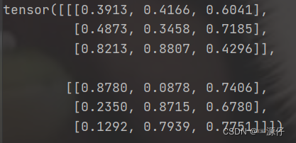
import torch.nn.functional as tnf
tnf.dropout(a,p=0.5)

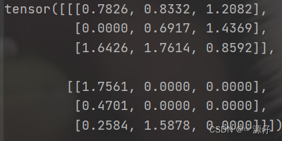
It can be found that the size of the above elements that are not 0 is twice the original size. That is, x.div(0.5), and then set it to 0 by random deactivation.

So why drop path should be implemented like this comes down to why dropout should be implemented like this, here is the explanation:

Assuming that the output activation value of a neuron is a, if dropout is not used, its output expectation value is a. If dropout is used, the neuron may have two states: reserved and closed, and it is regarded as a discrete random Variable, it conforms to the 0-1 distribution in probability theory, and the expectation of its output activation value becomes (1-p) a+p 0= (1-p)a. At this time, if you want to keep the expectation and not use dropout Consistent, it is necessary to divide by (1-p).

Explanation of the above code splitting:

import torch

drop_prob = 0.2
keep_prob = 1 - drop_prob
x = torch.randn(4, 3, 2, 2)
shape = (x.shape[0],) + (1,) * (x.ndim - 1)
random_tensor = keep_prob + torch.rand(shape, dtype=x.dtype, device=x.device)
random_tensor.floor_()
output = x.div(keep_prob) * random_tensor

OUT:

x.size():[4,3,2,2]
x：
tensor([[[[ 1.3833, -0.3703],
          [-0.4608,  0.6955]],
         [[ 0.8306,  0.6882],
          [ 2.2375,  1.6158]],
         [[-0.7108,  1.0498],
          [ 0.6783,  1.5673]]],

        [[[-0.0258, -1.7539],
          [-2.0789, -0.9648]],
         [[ 0.8598,  0.9351],
          [-0.3405,  0.0070]],
         [[ 0.3069, -1.5878],
          [-1.1333, -0.5932]]],

        [[[ 1.0379,  0.6277],
          [ 0.0153, -0.4764]],
         [[ 1.0115, -0.0271],
          [ 1.6610, -0.2410]],
         [[ 0.0681, -2.0821],
          [ 0.6137,  0.1157]]],

        [[[ 0.5350, -2.8424],
          [ 0.6648, -1.6652]],
         [[ 0.0122,  0.3389],
          [-1.1071, -0.6179]],
         [[-0.1843, -1.3026],
          [-0.3247,  0.3710]]]])

random_tensor.size():[4, 1, 1, 1]
random_tensor：
tensor([[[[0.]]],
        [[[1.]]],
        [[[1.]]],
        [[[1.]]]])

output.size():[4,3,2,2]
output：
tensor([[[[ 0.0000, -0.0000],
          [-0.0000,  0.0000]],
         [[ 0.0000,  0.0000],
          [ 0.0000,  0.0000]],
         [[-0.0000,  0.0000],
          [ 0.0000,  0.0000]]],

        [[[-0.0322, -2.1924],
          [-2.5986, -1.2060]],
         [[ 1.0748,  1.1689],
          [-0.4256,  0.0088]],
         [[ 0.3836, -1.9848],
          [-1.4166, -0.7415]]],

        [[[ 1.2974,  0.7846],
          [ 0.0192, -0.5955]],
         [[ 1.2644, -0.0339],
          [ 2.0762, -0.3012]],
         [[ 0.0851, -2.6027],
          [ 0.7671,  0.1446]]],

        [[[ 0.6687, -3.5530],
          [ 0.8310, -2.0815]],
         [[ 0.0152,  0.4236],
          [-1.3839, -0.7723]],
         [[-0.2303, -1.6282],
          [-0.4059,  0.4638]]]])

random_tensor is directly set to 0 as whether to keep the branch. If the probability of drop_path is set to 0.2, the number in random_tensor has a probability of 0.2, and the probability of being retained in output is 0.8.

Combined with the call of drop_path, if x is the input tensor and its channel is [B, C, H, W], then the meaning of drop_path is that in a Batch_size, there are randomly samples (fingers) of drop_prob, without going through the backbone, and Identity mapping directly by branch.

The above refers to the following two blogs ( I sincerely thank the two bloggers ):

• (Taking pytorch as an example) Simple understanding of the regularization method of path (depth)-drop path
• [Regularization] DropPath/drop_path usage

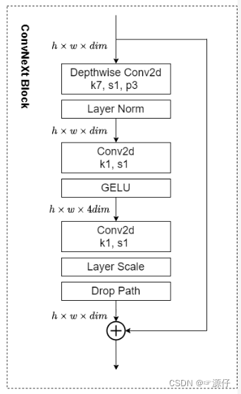
2、 Block

class Block(nn.Module):
    r""" ConvNeXt Block. There are two equivalent implementations:
    (1) DwConv -> LayerNorm (channels_first) -> 1x1 Conv -> GELU -> 1x1 Conv; all in (N, C, H, W)
    (2) DwConv -> Permute to (N, H, W, C); LayerNorm (channels_last) -> Linear -> GELU -> Linear; Permute back
    We use (2) as we find it slightly faster in PyTorch

    Args:
        dim (int): Number of input channels.
        drop_rate (float): Stochastic depth rate. Default: 0.0
        layer_scale_init_value (float): Init value for Layer Scale. Default: 1e-6.
    """
    def __init__(self, dim, drop_rate=0., layer_scale_init_value=1e-6):
        super().__init__()
        self.dwconv = nn.Conv2d(dim, dim, kernel_size=7, padding=3, groups=dim)  # 这里使用的是depthwise conv，group=channal数
        self.norm = LayerNorm(dim, eps=1e-6, data_format="channels_last")
        self.pwconv1 = nn.Linear(dim, 4 * dim)  # pointwise/1x1 convs, implemented with linear layers 
        self.act = nn.GELU()
        self.pwconv2 = nn.Linear(4 * dim, dim)  # 1乘1卷积等于全连接，作用是一样的
        # self.gamma:就是layer scale
        self.gamma = nn.Parameter(layer_scale_init_value * torch.ones((dim,)),
                                  requires_grad=True) if layer_scale_init_value > 0 else None
        self.drop_path = DropPath(drop_rate) if drop_rate > 0. else nn.Identity()

    def forward(self, x: torch.Tensor) -> torch.Tensor:
        shortcut = x
        x = self.dwconv(x)
        x = x.permute(0, 2, 3, 1)  # [N, C, H, W] -> [N, H, W, C]
        x = self.norm(x)
        x = self.pwconv1(x)
        x = self.act(x)
        x = self.pwconv2(x)
        if self.gamma is not None:
            x = self.gamma * x
        x = x.permute(0, 3, 1, 2)  # [N, H, W, C] -> [N, C, H, W]

        x = shortcut + self.drop_path(x)
        return x

3、 ConvNeXt

class ConvNeXt(nn.Module):
    r""" ConvNeXt
        A PyTorch impl of : `A ConvNet for the 2020s`  -
          https://arxiv.org/pdf/2201.03545.pdf
    Args:
        in_chans (int): Number of input image channels. Default: 3
        num_classes (int): Number of classes for classification head. Default: 1000
        depths (tuple(int)): Number of blocks at each stage. Default: [3, 3, 9, 3]
        dims (int): Feature dimension at each stage. Default: [96, 192, 384, 768]
        drop_path_rate (float): Stochastic depth rate. Default: 0.
        layer_scale_init_value (float): Init value for Layer Scale. Default: 1e-6.
        head_init_scale (float): Init scaling value for classifier weights and biases. Default: 1.
    """
    def __init__(self, in_chans: int = 3, num_classes: int = 1000, depths: list = None,
                 dims: list = None, drop_path_rate: float = 0., layer_scale_init_value: float = 1e-6,
                 head_init_scale: float = 1.):
        super().__init__()
        self.downsample_layers = nn.ModuleList()  # stem and 3 intermediate downsampling conv layers
        # stem :kernel  4,stride = 4
        stem = nn.Sequential(nn.Conv2d(in_chans, dims[0], kernel_size=4, stride=4),
                             LayerNorm(dims[0], eps=1e-6, data_format="channels_first"))
        self.downsample_layers.append(stem)

        # 对应stage2-stage4前的3个downsample(4个block之间连接的三个下采样)
        for i in range(3):
            downsample_layer = nn.Sequential(LayerNorm(dims[i], eps=1e-6, data_format="channels_first"),
                                             nn.Conv2d(dims[i], dims[i+1], kernel_size=2, stride=2))
            self.downsample_layers.append(downsample_layer)
		# self.downsample_layers中就包含了stem和三个下采样
		
        self.stages = nn.ModuleList()  # 4 feature resolution stages, each consisting of multiple blocks
        dp_rates = [x.item() for x in torch.linspace(0, drop_path_rate, sum(depths))]
        cur = 0
        # 构建每个stage中堆叠的block
        for i in range(4):
        	# 每个block乘以对应的depths=[3,3,9,3]
            stage = nn.Sequential(
                *[Block(dim=dims[i], drop_rate=dp_rates[cur + j], layer_scale_init_value=layer_scale_init_value)
                  for j in range(depths[i])]
            )
            self.stages.append(stage)
            cur += depths[i]

        self.norm = nn.LayerNorm(dims[-1], eps=1e-6)  # final norm layer
        self.head = nn.Linear(dims[-1], num_classes)
        self.apply(self._init_weights)
        self.head.weight.data.mul_(head_init_scale)
        self.head.bias.data.mul_(head_init_scale)

    def _init_weights(self, m):
        if isinstance(m, (nn.Conv2d, nn.Linear)):
            nn.init.trunc_normal_(m.weight, std=0.2)
            nn.init.constant_(m.bias, 0)

    def forward_features(self, x: torch.Tensor) -> torch.Tensor:
        for i in range(4):
            x = self.downsample_layers[i](x)
            x = self.stages[i](x)

        # global average pooling, (N, C, H, W) -> (N, C)
        return self.norm(x.mean([-2, -1]))  # x.mean([-2, -1])就是对H和W求均值，相当于平均池化


    def forward(self, x: torch.Tensor) -> torch.Tensor:
        x = self.forward_features(x)
        x = self.head(x)
        return x