Time series analysis steps and program details (python)
Article Directory
- Time series analysis steps and program details (python)
- foreword
- City's future mortality rate
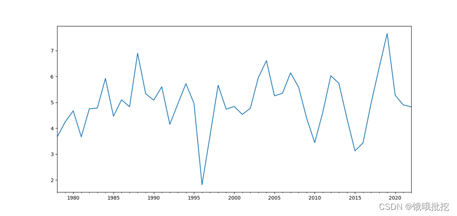
- 1. Draw the timing diagram of the sequence
- 2. Judging the stationarity and pure randomness of the sequence
- 3. Investigate the properties of the autocorrelation coefficient and partial autocorrelation coefficient of the sequence
- 4. Try to fit the development of the sequence with multiple models, and investigate the optimization problem of the fitting model of the sequence
- 5. Use the best fitting model to predict the population mortality rate of the city in the next 5 years.
foreword
Through the example of "Applied Time Series Analysis (6th Edition)" Wang Yan's time series two example questions 4.4 and 4.7, the following are all python programming, time series codes in other languages can chat with me privately.
Note: The code will not run the subsequent code if the code does not cross out the picture. If there is no picture, you can add a plt.show()
City's future mortality rate
Import the third-party library first
clear;clc
from __future__ import print_function
import pandas as pd
import numpy as np
from scipy import  stats
import matplotlib.pyplot as plt
import statsmodels.api as sm
from statsmodels.graphics.api import qqplot
from statsmodels.stats.diagnostic import acorr_ljungbox
Import Data
data=pd.Series([3.665,4.247,4.674,3.669,4.752,4.785,5.929,4.468,5.102,4.831,6.899,5.337,5.086,
      5.603,4.153,4.945,5.726,4.965,1.82,3.723,5.663,4.739,4.845,4.535,4.774,5.962,
      6.614,5.255,5.355,6.144,5.59,4.388,3.447,4.615,6.032,5.74,4.391,3.128,3.436,
      4.964,6.332,7.665,5.277,4.904,4.83,])
1. Draw the timing diagram of the sequence
data=pd.Series(data)
data.index = pd.Index(sm.tsa.datetools.dates_from_range('1978','2022'))
data.plot(figsize=(12,8))
2. Judging the stationarity and pure randomness of the sequence
(i) Stationarity test
# ADF单位根平稳型检验
ADF = sm.tsa.stattools.adfuller(data)
print(ADF[0:2]) #输出统计量和对应的p值
if ADF[4]['1%'] > ADF[0]:
      print('ADF单位根平稳型检验通过,显著的拒绝原假设,数据是平稳的')
else:
      print('ADF单位根平稳型检验不通过,接受原假设,数据是不平稳的')
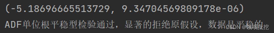
Significance level 1%, %5, 10% different degrees of rejection of the statistical value of the original hypothesis and the comparison of ADF Test result, ADF Test result is less than 1%, 5%, 10% at the same time, which means that the hypothesis is rejected very well, this data Among them, the adf result is -5.18696, which is less than the statistical value of three levels. It is less than the statistical critical value corresponding to the significance level of 0.01 -3.59250. The corresponding P value is very close to 0. In this data, the P value is 9e-6, which is close to 0.
If you do not pass the stationarity test, you need to perform a difference. The difference code is as follows
#一阶差分
fig = plt.figure(figsize=(12,8))
ax1= fig.add_subplot(111)
diff1 = data.diff(1)
diff1.plot(ax=ax1)

#二阶差分
fig = plt.figure(figsize=(12,8))
ax2= fig.add_subplot(111)
diff2 = data.diff(2)
diff2.plot(ax=ax2)
(ii) Pure randomness test
# 白噪声检验
bzs = acorr_ljungbox(data.dropna(), lags = [i for i in range(1,12)],boxpierce=True)
print(bzs)
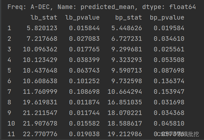
The second line here is the p value, which corresponds to the p value corresponding to each autoregressive coefficient. If all of them are greater than 0.05, then this sequence is a white noise sequence and has no value.
3. Investigate the properties of the autocorrelation coefficient and partial autocorrelation coefficient of the sequence
# 检查平稳时间序列的自相关图和偏自相关图
dta= data.diff(1)#我们已经知道要使用一阶差分的时间序列,之前判断差分的程序可以注释掉
fig = plt.figure(figsize=(12,8))
ax1=fig.add_subplot(211)
fig = sm.graphics.tsa.plot_acf(data,title="ACF",ax=ax1)
ax2 = fig.add_subplot(212)
fig = sm.graphics.tsa.plot_pacf(data,title="PACF",ax=ax2,method='ywm')
plt.show()
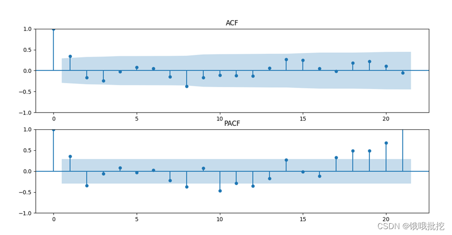
It is not difficult to see that according to the sequence autocorrelation graph, it can be regarded as: the first-order truncation of the autocorrelation graph, or the second-order truncation of the partial autocorrelation.
It can also be considered that the autocorrelation graph is first-order truncated, and the partial autocorrelation is tailed.
4. Try to fit the development of the sequence with multiple models, and investigate the optimization problem of the fitting model of the sequence
According to autocorrelation and partial autocorrelation, select the corresponding model, here choose MA(1), AR(2), ARMA(1,1)
#参数检验
model1 = sm.tsa.arima.ARIMA(data, order=(0,0,1))
result1 = model1.fit()
model2 = sm.tsa.arima.ARIMA(data, order=(2,0,0))
result2 = model2.fit()
model3 = sm.tsa.arima.ARIMA(data, order=(1,0,1))
result3 = model3.fit()
print(result1.summary())
print(result2.summary())
print(result3.summary())
print('arma(1,1)参数检验存在问题,参数显著为零,淘汰arma(1,1)')
print('MA(1),AR(2)参数显著非零,残差检验均为白噪声序列,MA(1)模型在AIC和BIC更优,所以选择MA(1)为最优模型')
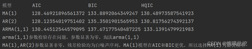
#AIC BIC HQIC
print('模型 ','AIC ','BIC ','HQIC ')
print('MA(1) ',arma_mod20.aic,arma_mod20.bic,arma_mod20.hqic)
print('AR(2) ',arma_mod30.aic,arma_mod30.bic,arma_mod30.hqic)
print('ARMA(1,1)',arma_mod40.aic,arma_mod40.bic,arma_mod40.hqic)
Output results (aic and bic comparison of each model):
parameter inspection of each model (only unqualified arma(1,1) is placed here)
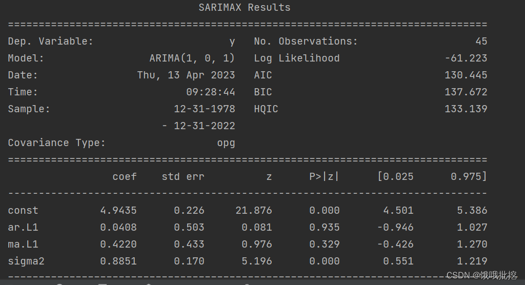
There is a problem with the ARMA(1,1) parameter test, the parameter is significantly zero, and the ARMA(1,1) model
MA(1), AR(2) parameter is significantly non-zero, the residual test is a white noise sequence, MA(1 ) model is better in AIC and BIC, so choose MA(1) as the optimal model (the bigger the aic and bic, the better)
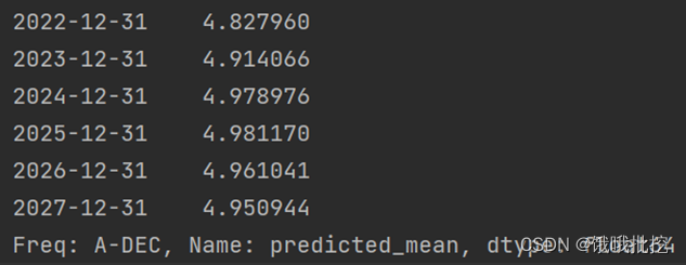
5. Use the best fitting model to predict the population mortality rate of the city in the next 5 years.
pred = result1.predict('2022','2027',dynamic=True, typ='levels')
print (pred)
The above code, if there is any similarity, is purely a brick