Build machine learning applications with Amazon SageMaker
Watch the full deployment video here. The original video is about 30 minutes long and the waiting time has been cut for viewing experience:
Xiaobai uses Amazon SageMaker to build machine learning applications
1. Create a Sagemaker Notebook instance
Amazon SageMaker: https://aws.amazon.com/cn/sagemaker/Enter
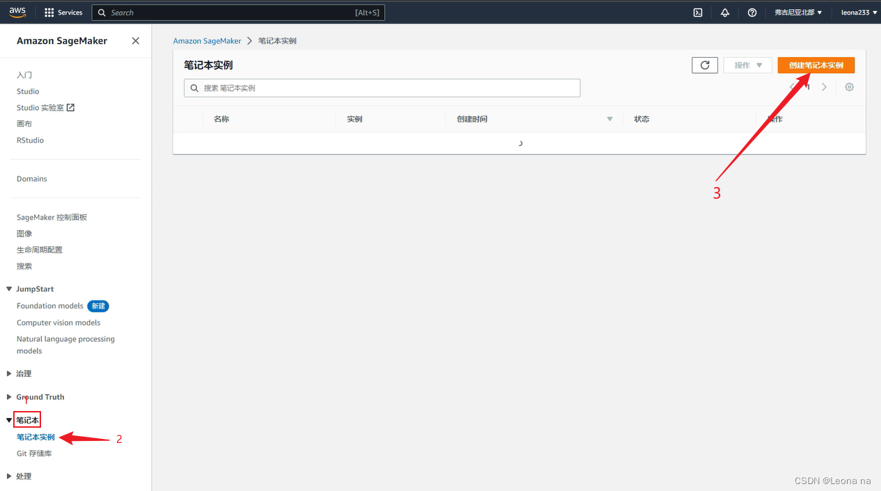
the name, select the instance type, and configure the disk size, as shown in the figure below
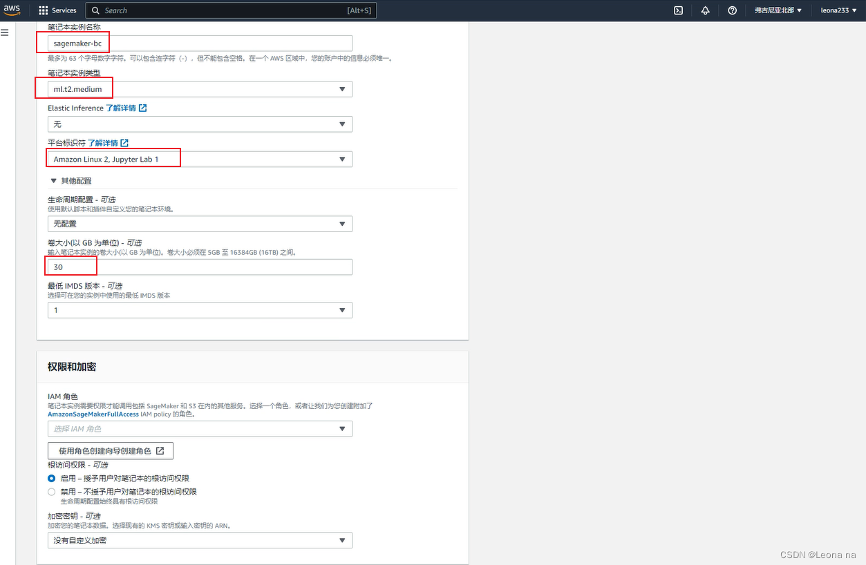
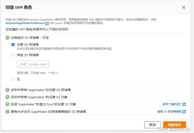
Create a new role, select any S3 bucket, click Create role

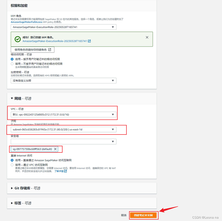
to configure the VPC network, and select VPC , subnet and security group, and click to create a notebook instance
Wait for 5-6 minutes, the status changes to inSerice, click to open jupyter

to create a new file, as shown below

2. Download the dataset
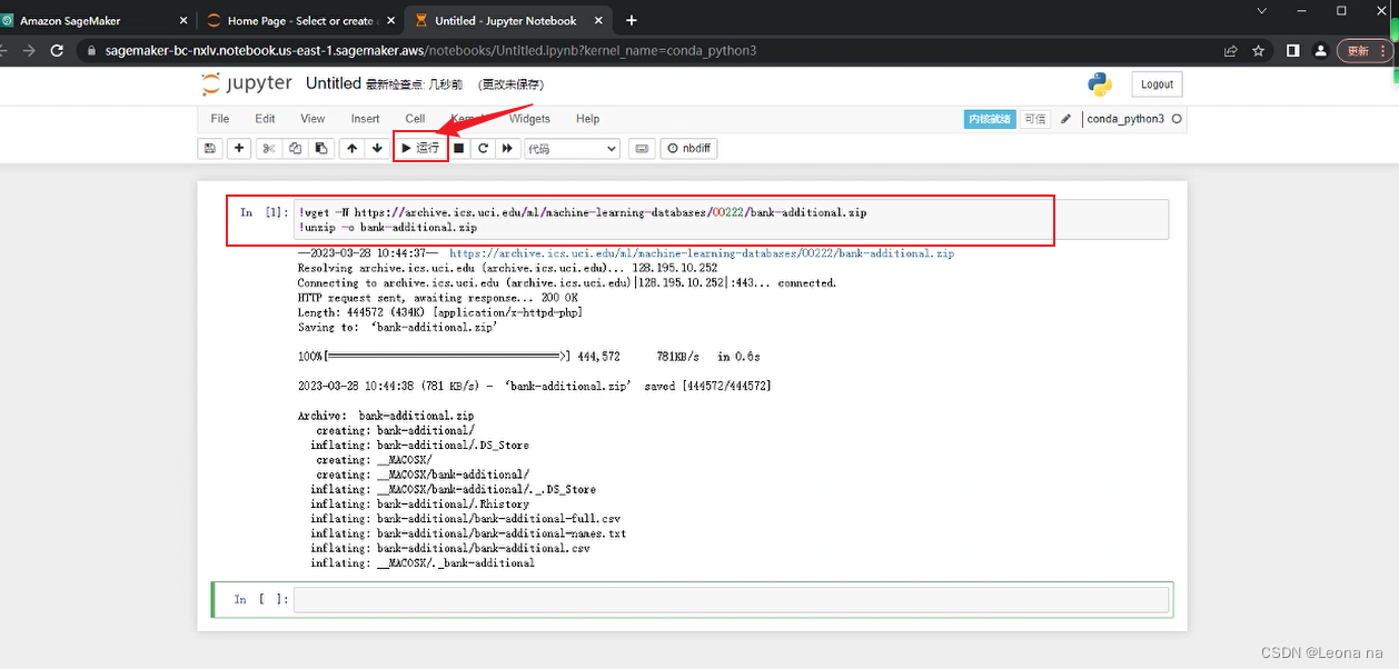
Enter the following code to download the dataset and decompress it:
!wget -N https://archive.ics.uci.edu/ml/machine-learning-databases/00222/bank-additional.zip
!unzip -o bank-additional.zip
After pasting the code, click Run
Display datasets through pandas
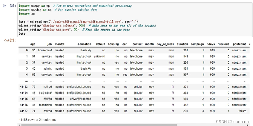
Use the bank-additional-full.csv dataset file, read it in and display it through pandas:
import numpy as np  # For matrix operations and numerical processing
import pandas as pd  # For munging tabular data
import os

data = pd.read_csv("./bank-additional/bank-additional-full.csv", sep=";")
pd.set_option("display.max_columns", 500)  # Make sure we can see all of the columns
pd.set_option("display.max_rows", 50)  # Keep the output on one page
data
The features are explained as follows:

3. Data preprocessing
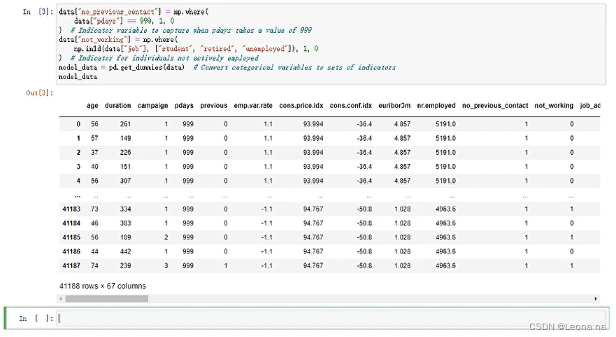
Data cleaning converts categorical data into numbers by one-hot encoding.
data["no_previous_contact"] = np.where(
    data["pdays"] == 999, 1, 0
)  # Indicator variable to capture when pdays takes a value of 999
data["not_working"] = np.where(
    np.in1d(data["job"], ["student", "retired", "unemployed"]), 1, 0
)  # Indicator for individuals not actively employed
model_data = pd.get_dummies(data)  # Convert categorical variables to sets of indicators
model_data
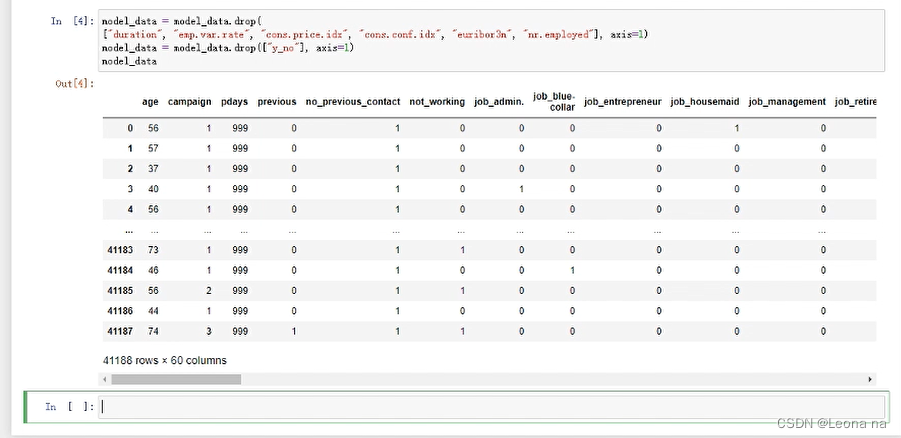
Delete related features and duration features in the data
model_data = model_data.drop(
["duration", "emp.var.rate", "cons.price.idx", "cons.conf.idx", "euribor3m", "nr.employed"], axis=1)
model_data = model_data.drop(["y_no"], axis=1)
model_data
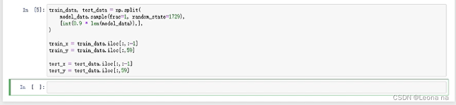
Split the dataset into training (90%) and test (10%) datasets, and convert the datasets into the correct format that the algorithm expects. The training dataset is used during training and these test datasets will be used to evaluate the model performance after the model training is complete.
4. Use XGBoost to train the model
Install XGBoost
!pip install xgboost
Using the python XGBoost API
Start model training, and save the model when complete. Then the previously reserved test data set is sent to the model for inference. We regard the inference result greater than the threshold (0.5) as 1, otherwise it is 0, and then compare it with the labels in the test set to evaluate the effect of the model.
import numpy as np
import pandas as pd
import xgboost as xgb
from sklearn.model_selection import train_test_split

# 用sklearn.cross_validation进行训练数据集划分,这里训练集和交叉验证集比例为8:2,可以自己根据需要设置
X, val_X, y, val_y = train_test_split(
    train_x,
    train_y,
    test_size=0.2,
    random_state=2022,
    stratify=train_y
)

# xgb矩阵赋值
xgb_val = xgb.DMatrix(val_X, label=val_y)
xgb_train = xgb.DMatrix(X, label=y)
xgb_test = xgb.DMatrix(test_x)

# xgboost模型 #####################
params = {
    'booster': 'gbtree',
    'objective': 'binary:logistic',
    'eval_metric': 'auc', #logloss
    'gamma': 0.1,  # 用于控制是否后剪枝的参数,越大越保守,一般0.1、0.2
    'max_depth': 8,  # 构建树的深度,越大越容易过拟合
    'alpha': 0,   # L1正则化系数
    'lambda': 10,  # 控制模型复杂度的权重值的L2正则化项参数,参数越大,模型越不容易过拟合
    'subsample': 0.7,  # 随机采样训练样本
    'colsample_bytree': 0.5,  # 生成树时进行的列采样
    'min_child_weight': 3,
    # 这个参数默认是 1,是每个叶子里面 h 的和至少是多少,对正负样本不均衡时的 0-1 分类而言
    # ,假设 h 在 0.01 附近,min_child_weight 为 1 意味着叶子节点中最少需要包含 100 个样本。
    # 这个参数非常影响结果,控制叶子节点中二阶导的和的最小值,该参数值越小,越容易 overfitting。
    'silent': 0,  # 设置成1则没有运行信息输出,最好是设置为0.
    'eta': 0.03,  # 如同学习率
    'seed': 1000,
    'nthread': -1,  # cpu 线程数
    'missing': 1,
    'scale_pos_weight': (np.sum(y==0)/np.sum(y==1))  # 用来处理正负样本不均衡的问题,通常取:sum(negative cases) / sum(positive cases)
}

plst = list(params.items())
num_rounds = 500  # 迭代次数
watchlist = [(xgb_train, 'train'), (xgb_val, 'val')]

# 训练模型并保存
# early_stopping_rounds 当设置的迭代次数较大时,early_stopping_rounds 可在一定的迭代次数内准确率没有提升就停止训练
model = xgb.train(plst, xgb_train, num_rounds, watchlist, early_stopping_rounds=200)
model.save_model('./xgb.model')  # 用于存储训练出的模型

preds = model.predict(xgb_test)

# 导出结果
threshold = 0.5
ypred = np.where(preds > 0.5, 1, 0)

from sklearn import metrics

print ('AUC: %.4f' % metrics.roc_auc_score(test_y,ypred))
print ('ACC: %.4f' % metrics.accuracy_score(test_y,ypred))
print ('Recall: %.4f' % metrics.recall_score(test_y,ypred))
print ('F1-score: %.4f' %metrics.f1_score(test_y,ypred))
print ('Precesion: %.4f' %metrics.precision_score(test_y,ypred))
print(metrics.confusion_matrix(test_y,ypred))
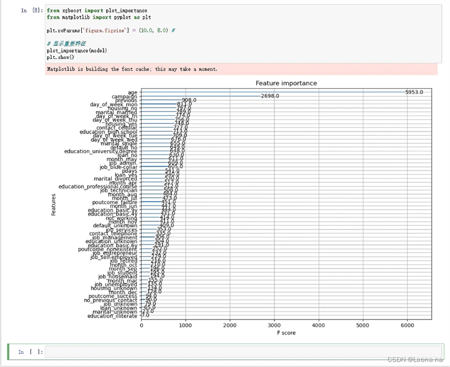
Outputs the importance of different features in the model, which usually helps us better understand the behavior of the model.
from xgboost import plot_importance
from matplotlib import pyplot as plt

plt.rcParams['figure.figsize'] = (10.0, 8.0) #

# 显示重要特征
plot_importance(model)
plt.show()
5. Use SageMaker Training API to carry out model training
initialization
import sagemaker
import boto3

import numpy as np  # For matrix operations and numerical processing
import pandas as pd  # For munging tabular data
from time import gmtime, strftime
import os

region = boto3.Session().region_name
smclient = boto3.Session().client("sagemaker")

role = sagemaker.get_execution_role()

bucket = sagemaker.Session().default_bucket()
prefix = "sagemaker/DEMO-hpo-xgboost-dm"
data processing
data = pd.read_csv("./bank-additional/bank-additional-full.csv", sep=";")
pd.set_option("display.max_columns", 500)  # Make sure we can see all of the columns
data["no_previous_contact"] = np.where(
    data["pdays"] == 999, 1, 0
)  # Indicator variable to capture when pdays takes a value of 999
data["not_working"] = np.where(
    np.in1d(data["job"], ["student", "retired", "unemployed"]), 1, 0
)  # Indicator for individuals not actively employed
model_data = pd.get_dummies(data)  # Convert categorical variables to sets of indicators
model_data = model_data.drop(
    ["duration", "emp.var.rate", "cons.price.idx", "cons.conf.idx", "euribor3m", "nr.employed"],
    axis=1,

)
Split the dataset into training (70%), validation (20%), and test (10%) datasets, and convert the dataset to the correct format expected by SageMaker's built-in XGBoost algorithm. We will use training and validation datasets during training. The test dataset will be used to evaluate the model performance after being deployed to the endpoint.
train_data, validation_data, test_data = np.split(
    model_data.sample(frac=1, random_state=1729),
    [int(0.7 * len(model_data)), int(0.9 * len(model_data))],
)

pd.concat([train_data["y_yes"], train_data.drop(["y_no", "y_yes"], axis=1)], axis=1).to_csv(
    "train.csv", index=False, header=False
)
pd.concat(
    [validation_data["y_yes"], validation_data.drop(["y_no", "y_yes"], axis=1)], axis=1
).to_csv("validation.csv", index=False, header=False)
pd.concat([test_data["y_yes"], test_data.drop(["y_no", "y_yes"], axis=1)], axis=1).to_csv(
    "test.csv", index=False, header=False
)
Upload the generated dataset to S3 for use in the next step of model training.
boto3.Session().resource("s3").Bucket(bucket).Object(
    os.path.join(prefix, "train/train.csv")
).upload_file("train.csv")
boto3.Session().resource("s3").Bucket(bucket).Object(
    os.path.join(prefix, "validation/validation.csv")
).upload_file("validation.csv")


from sagemaker.inputs import TrainingInput

s3_input_train = TrainingInput(
    s3_data="s3://{}/{}/train".format(bucket, prefix), content_type="csv"
)
s3_input_validation = TrainingInput(
    s3_data="s3://{}/{}/validation/".format(bucket, prefix), content_type="csv"
)
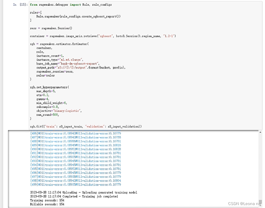
Generate XGBoost model training report, it will be slower here
from sagemaker.debugger import Rule, rule_configs

rules=[
    Rule.sagemaker(rule_configs.create_xgboost_report())
]

sess = sagemaker.Session()

container = sagemaker.image_uris.retrieve("xgboost", boto3.Session().region_name, "1.2-1")

xgb = sagemaker.estimator.Estimator(
    container,
    role,
    instance_count=1,
    instance_type="ml.m4.xlarge",
    base_job_name="bank-dm-xgboost-report",
    output_path="s3://{}/{}/output".format(bucket, prefix),
    sagemaker_session=sess,
    rules=rules
)

xgb.set_hyperparameters(
    max_depth=5,
    eta=0.2,
    gamma=4,
    min_child_weight=6,
    subsample=0.8,
    objective="binary:logistic",
    num_round=500,
)

xgb.fit({"train": s3_input_train, "validation": s3_input_validation})
The output result is as follows
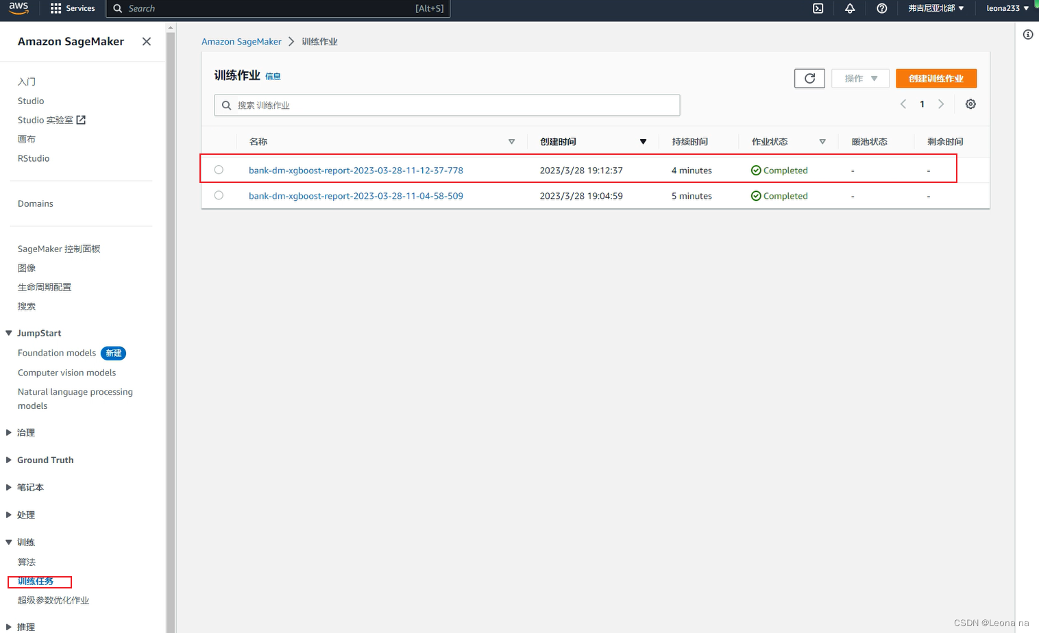
6. Training task management
Find the SageMaker console-training-training task
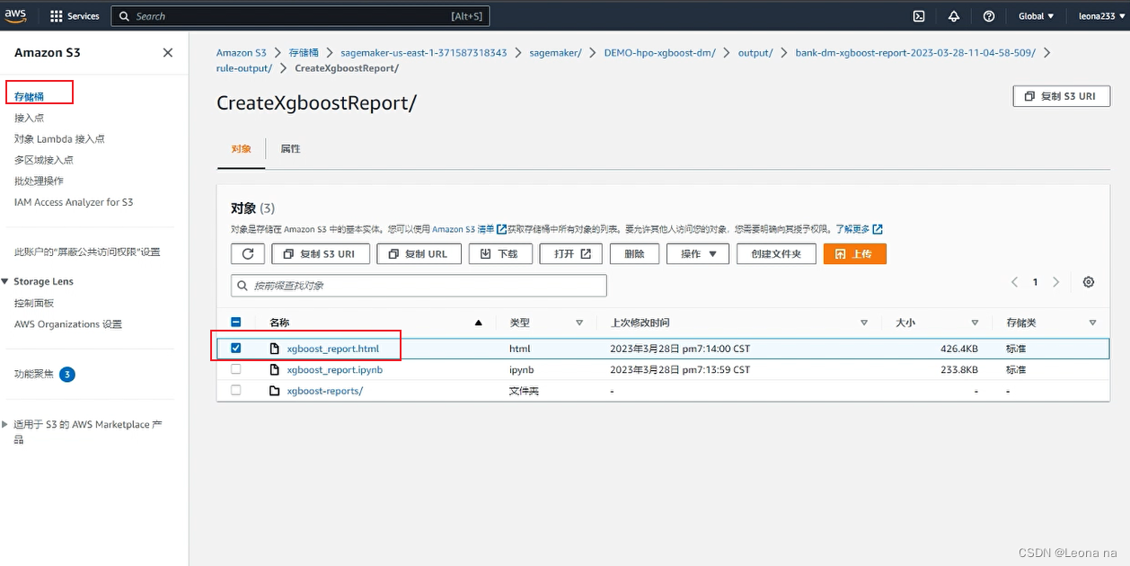
Training report S3 storage location
7. AutoGluon training model
AutoGluon installation
# Install AutoGluon
!pip install -U setuptools wheel
!pip install -U "mxnet<2.0.0"
!pip install autogluon
Train the model with AutoGluon Tabular
from autogluon.tabular import TabularDataset, TabularPredictor
ag_data = pd.read_csv("./bank-additional/bank-additional-full.csv", sep=";")
label = 'y'
print("Summary of y variable: \n", ag_data[label].describe())

ag_train_data, ag_test_data = np.split(
    ag_data.sample(frac=1, random_state=1729),
    [int(0.9 * len(model_data)),],
)
Using AutoGluon, we don't need to do data processing (missing value processing, one-hot encoding, etc.), AutoGloun will automatically do these tasks for us.
ag_test_data_X = ag_test_data.iloc[:,:-1]
ag_test_data_y =ag_test_data.iloc[:,20]

save_path = 'agModels-predictClass'  # specifies folder to store trained models

learner_kwargs = {'ignored_columns':[["duration", "emp.var.rate", "cons.price.idx", "cons.conf.idx", "euribor3m", "nr.employed"]]}

predictor = TabularPredictor(label=label, path=save_path,
                             eval_metric='recall', learner_kwargs=learner_kwargs
                            ).fit(ag_train_data)
predictor = TabularPredictor.load(save_path)  # unnecessary, just demonstrates how to load previously-trained predictor from file

ag_y_pred = predictor.predict(ag_test_data_X)
ag_y_pred_proa = predictor.predict_proba(ag_test_data_X)

print("Predictions:  \n", ag_y_pred)
perf = predictor.evaluate_predictions(y_true=ag_test_data_y, y_pred=ag_y_pred, auxiliary_metrics=True)
# perf = predictor.evaluate_predictions(y_true=ag_test_data_y, y_pred=ag_y_pred_proa, auxiliary_metrics=True) #when eval_metric='auc' in TabularPredictor()
After the experiment is over, remember to stop the instance and delete all relevant content such as roles, policies, log groups, etc.
8. Summary
The entire experiment is deployed with reference to the Amazon official manual, and the process is relatively simple. But the access speed is very slow. Sometimes half of the execution will get stuck and need to be re-executed. I hope Amazon can improve the slow network problem, which will affect the user experience a bit. Sagemaker is very convenient. Jupyter Notebook and Notebook instances provide several development environments such as PyTorch, Numpy, Pandas, etc., which reduces the time and cost of installation. I, a novice who has never learned machine learning, can quickly start building. Lowering the threshold for machine learning. I have learned a lot from this experiment, and the deployment is only the first step. For details, I need to read the official deployment manual several times to digest.
9. References
Reference article: Amazon Cloud Technology [Cloud Exploration Lab] Use Amazon SageMaker to build machine learning applications, build fine-grained sentiment analysis applications, and quickly build your first AIGC application based on the Stable Diffusion model
Deployment article: https://dev .amazoncloud.cn/column/article/63ff329f4891d26f36585a9c