1. Conjugate gradient method
For the textbook calculation example P113: use the conjugate gradient method to solve the linear equation system Ax=b, where the
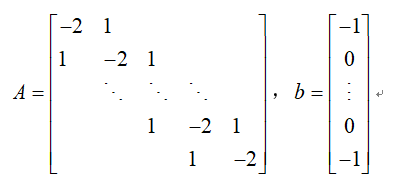
order n of the matrix A is taken as 100, 200, 400 respectively, and point out whether the calculation results are reliable.
The solution results of the conjugate gradient method are as follows:
(1) When n=100,
the accuracy requirement is met after 50 iterations, and the error curve is shown in the figure below.

(2) When n=200,
the accuracy requirement is met after 100 iterations, and the error curve is shown in the figure below.

(2) When n=400,
the accuracy requirement is met after 200 iterations, and the error curve is shown in the figure below.

(1) The reliability of the result is
n=100, the iteration is 50 times, the error decreases rapidly, reaching 1.07 10-12, and the final result x=(1 1 ... 1)T is brought into the equation, which conforms to the meaning of the question.
n=200, 100 iterations, the error decreases rapidly, reaching 6.23 10-12, the final result x=(1 1 ... 1)T, brought into the equation, conforms to the meaning of the question.
n=400, 200 iterations, the error decreases rapidly, reaching 2.14*10-11, the final result x=(1 1 ... 1)T, brought into the equation, conforms to the meaning of the question.
(2) Advantages
It is suitable for symmetric matrix operations with simple structure, high consistency and large order.
(3) Limitations
This algorithm is only applicable to sparse symmetric arrays with consistent diagonal elements of A, and not applicable to inconsistent diagonal elements. Likewise, the resulting b vector is suitable for cases where individual elements are nonzero and others are zero.
Second, the steepest descent method
(1) When n=100,
when the precision is 1*10-6, it takes 19465 iterations to meet the precision requirement.

(2) When n=200,
when the precision is 1*10-6, it takes 68688 iterations to meet the precision requirement.

(3) When n=400,
when the precision is 1*10-6, it takes 239671 iterations to meet the precision requirement.

From the above results, it can be seen that the number of iterations of the steepest descent method is much higher than that of the conjugate gradient method when the same accuracy is satisfied.
Third, the comparison between the two
Taking n=200 as an example, draw the curve of the error of the conjugate gradient method and the steepest descent method with the number of iterations, as shown in the figure below. 
The analysis shows that when the number of iterations of the conjugate gradient method reaches n, the error will decrease rapidly, while the trend of the steepest descent method error reduction is relatively flat, indicating that its convergence speed is slow.