Article Directory
illustrate
Many of the enlarged circuit diagrams in the book are theoretical diagrams, which are different from actual applications. For example, the following non-inverting amplifier circuit:

There is no problem in theoretical analysis, but the diagram of our actual application should be as follows:
it is necessary to add an additional freewheeling resistor. If there is no freewheeling resistor, the capacitor at the positive end of the amplifier has no current input and cannot work. Therefore, this article is based on proteus simulation, and this article is made to record the amplifier circuit in practical applications. Among them, each channel of the oscilloscope is named OS1, OS2, etc., and OS1, etc. appearing in the circuit of this article means that it is connected to channel 1 of the oscilloscope.
Non-inverting amplifier circuit
The theoretical diagram is as follows:

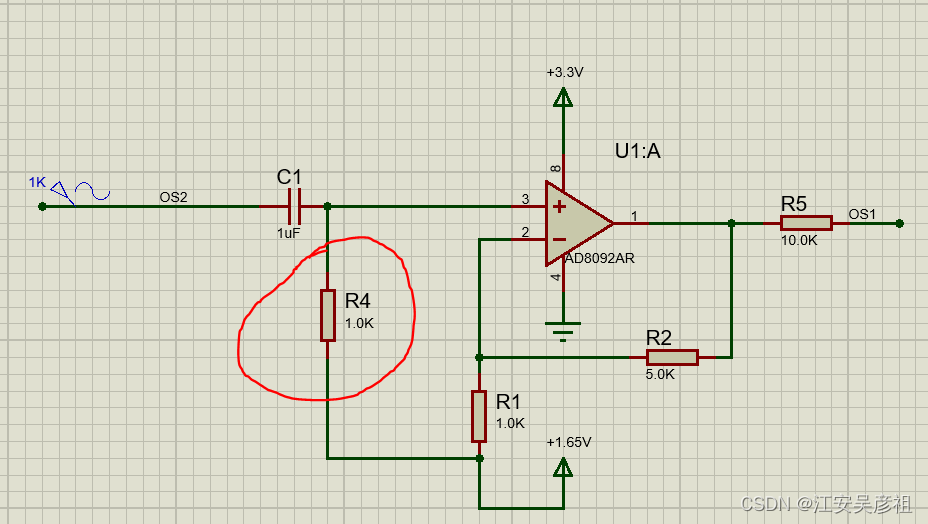
the actual diagram is as follows:
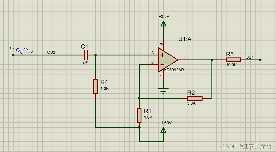
where capacitor C1 is the coupling input capacitor, if its value is relatively small, according to the capacitance impedance formula: the smaller the
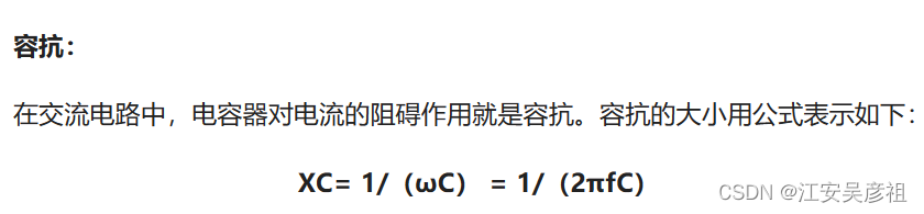
capacitance value, the larger its capacitive reactance, and only higher frequency signals can pass through.
And if the capacitance value is selected too large, the low-frequency noise signal can also pass through.
reverse amplifier circuit
As follows:
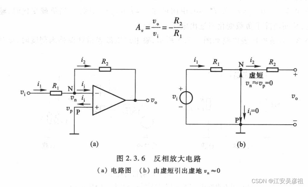
The actual circuit diagram is as follows:
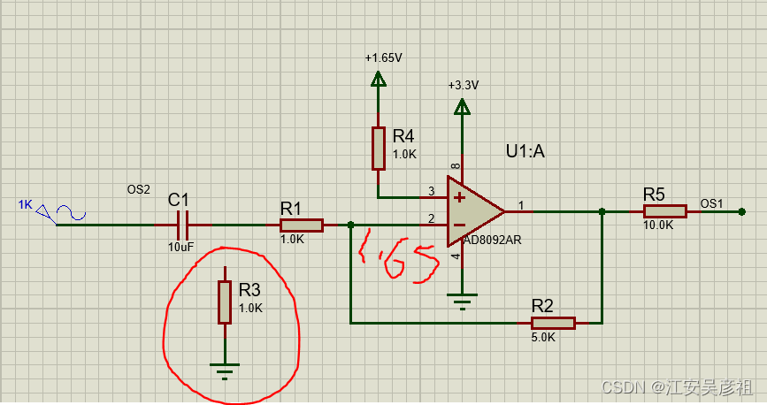
Note: At this time, the freewheeling resistor R3 cannot be added, and the capacitor C1 is charged through R1.
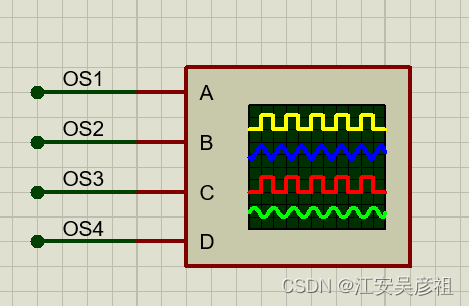
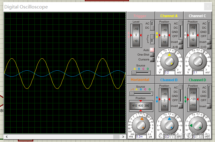
The effect is as follows:
amplifier filter circuit
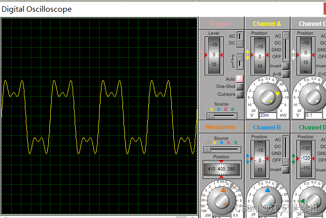
An important application of the amplifier is the filtering effect. We assume that the following three sinusoidal signals are mixed together, as shown in the figure below:
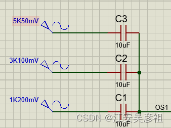
Among them, 5K50mV means that the frequency is 5KHZ and the amplitude is 50mV. Then its shape in the oscilloscope is as follows:
We choose various filter circuits to restore the signal below.
low pass filter circuit
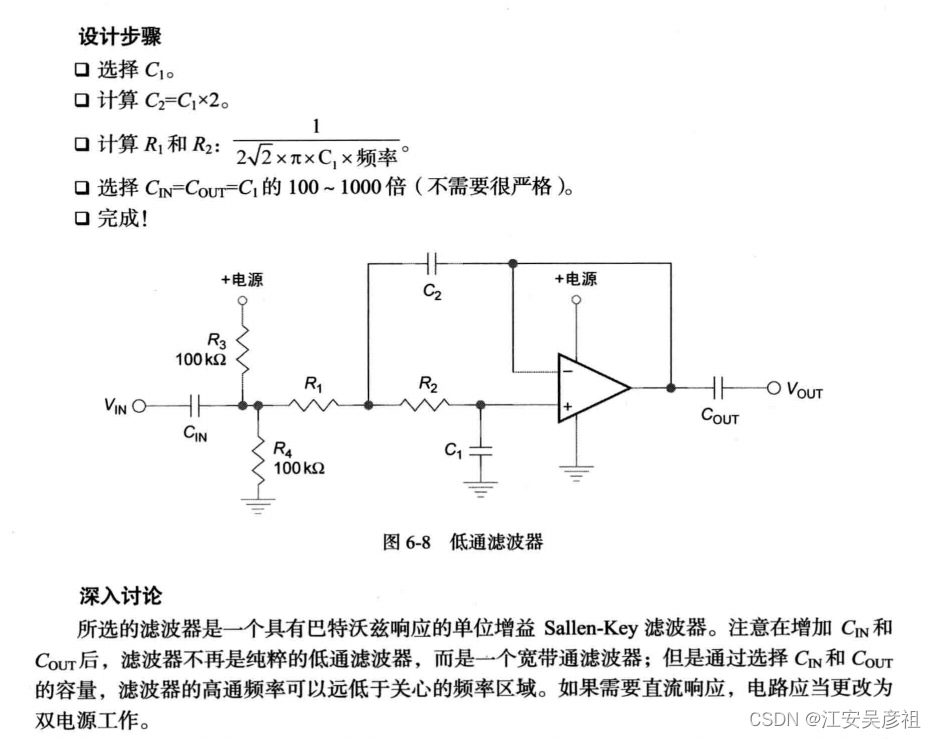
The actual circuit diagram is as follows:
we choose the cutoff frequency of the filter to be 1khz, then:
R 1 × C 1 = 1 2 2 × π × f R_1 \times C_1 =\frac{1}{2 \sqrt{2} \times \pi \times f}R1×C1=22×π×f1
Substituting f=1000HZ, then:
R 1 × C 1 = 1 8.8857 × f = 1 8885.7 = 1.125 × 1 0 − 4 R_1 \times C_1 =\frac{1}{8.8857 \times f}=\frac{1}{ 8885.7}=1.125 \times 10^{-4}R1×C1=8.8857×f1=8885.71=1.125×10⁻⁴
Choose R1=R2=100 Ω \OmegaΩ
则 C1= 1.125 × 1 0 − 6 F = 1.125 u F 1.125 \times 10^{-6}F=1.125uF 1.125×10⁻⁶ F _=1.125 uF Since the capacitance value is generally discontinuous and the accuracy is not as high as that
of the resistor, and the resistor is optional, it is interchangeable:
R1=R2=112.5Ω \OmegaΩ
则 C1= 1 × 1 0 − 6 F = 1 u F 1 \times 10^{-6}F=1 uF 1×10⁻⁶ F _=1uF
则 C2= 2 × 1 0 − 6 F = 2 u F 2 \times 10^{-6}F=2 uF 2×10⁻⁶ F _=2 u F
proteus simulation
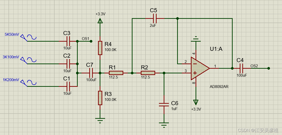
At this time, the proteus simulation effect is as follows:

the yellow color is the input signal, including 1K, 3K, and 5K sine waves. Blue is the filtered signal, we found its frequency is 1us. Therefore, the filter circuit design is correct.
In addition, you can also use more professional analog simulation software: choose TINA TI here, the software is only 100M in size, and you can easily analyze the circuit response.
TINA TI Simulation
As shown in the figure below is a 500KHZ low-pass filter, the source is the OPA357 data sheet:
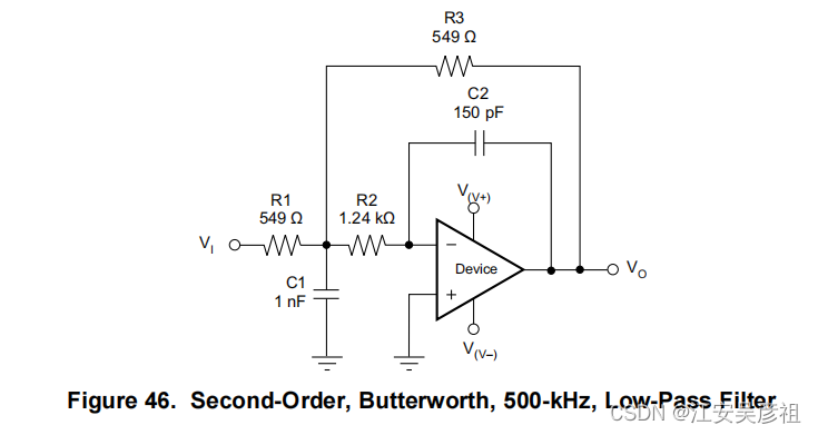
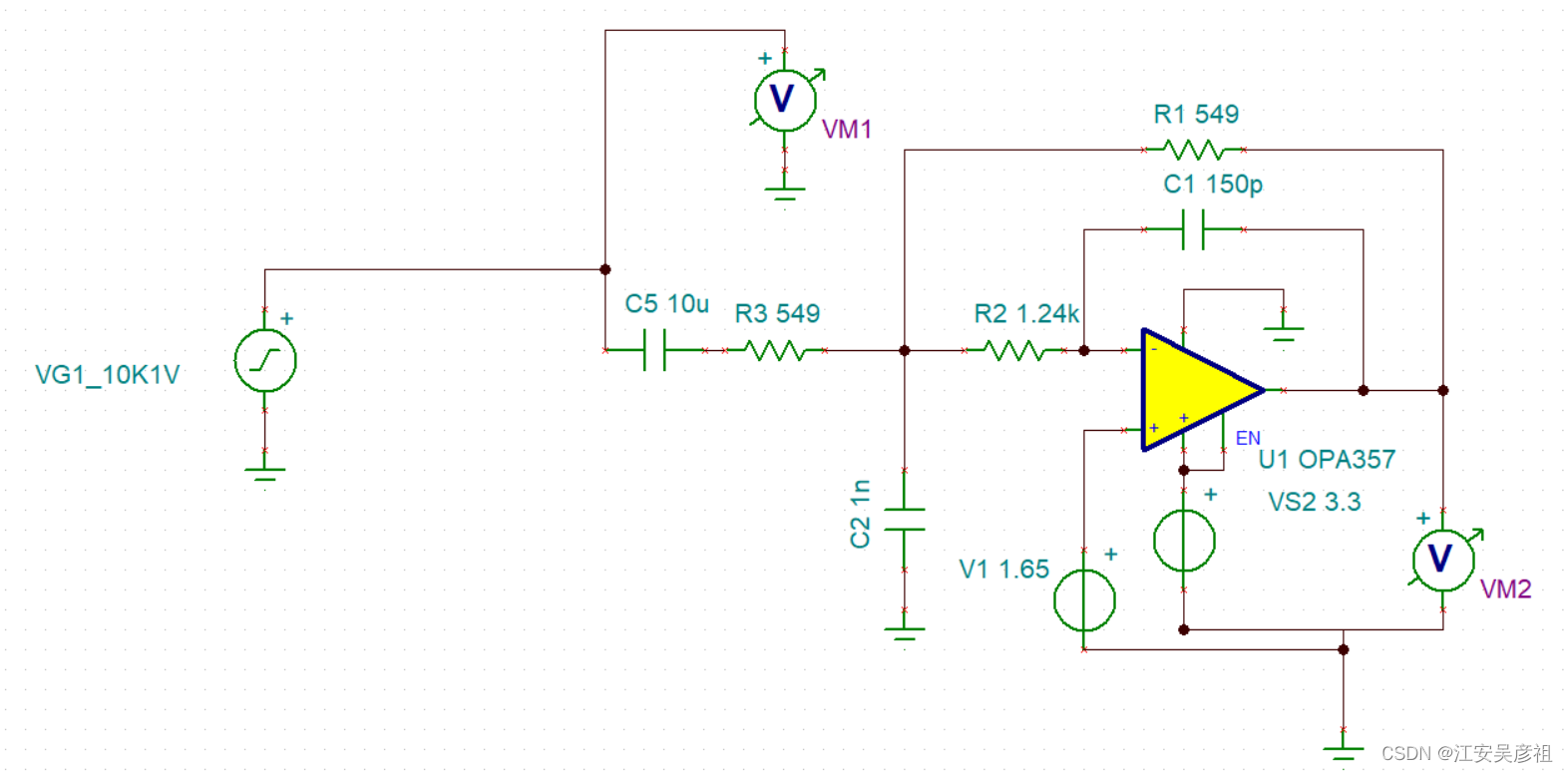
We analyze the circuit response as follows:
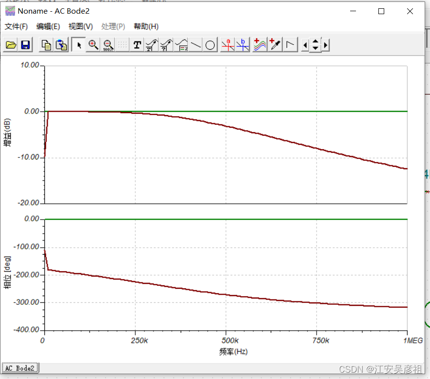
the input signal is a 50KHZ square wave, then the input and output signals are:
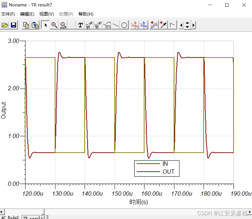
It can be found that the software is particularly convenient for designing filters.
We design our above circuit in proteus and analyze its circuit response:
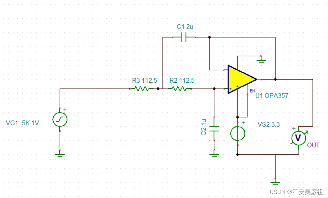
The analysis results are as follows:
It can be seen that for the 5KHZ signal, the filtering effect is relatively good.
For 1KHZ signals, it is slightly attenuated.
For the 500HZ signal, there is basically no attenuation.
Analyze its frequency domain characteristics: you can find its better low-pass filtering characteristics.
narrowband filter circuit
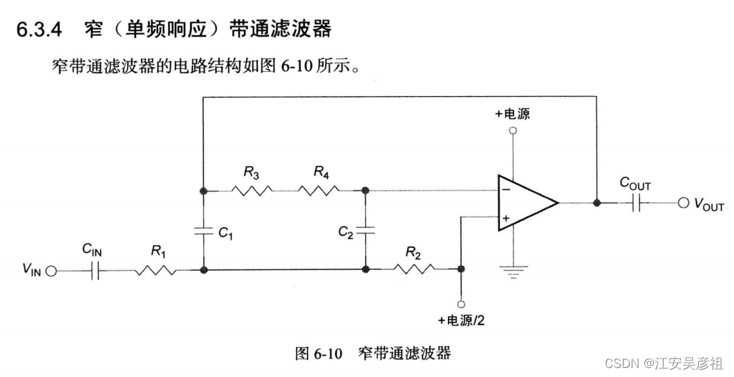
preteus simulation
Similarly, we design a 3KHZ narrowband filter circuit to filter 3K out of 1K, 3K, 5K and other signals.
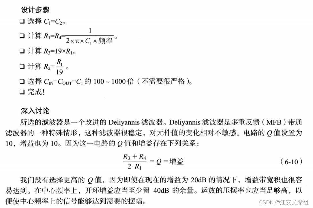
We choose the passband frequency of the filter to be 3khz, then:
R 1 × C 1 = 1 2 × π × f R_1 \times C_1 =\frac{1}{2 \times \pi \times f}R1×C1=2×π×f1
Substitute f=3000HZ, then:
R 1 × C 1 = 1 6.28318 × f = 1 18849.54 = 5.305 × 1 0 − 5 R_1 \times C_1 =\frac{1}{6.28318 \times f}=\frac{1}{18849.54}=5.305 \times 10^{-5} R1×C1=6.28318×f1=18849.541=5.305×10⁻⁵
Choose R1=R2=100 Ω \OmegaΩ
则 C1= 5.305 × 1 0 − 7 F = 0.5305 u F 5.305 \times 10^{-7}F=0.5305uF 5.305×10⁻⁷ F _=0.5305 uF
Because the capacitance value is generally discontinuous and the precision is not as high as that of the resistor, and the resistor is optional, so it is interchangeable: R1
=R4=530.5Ω \OmegaΩ
则 C1= 1 × 1 0 − 7 F = 0.1 u F 1 \times 10^{-7}F=0.1 uF 1×10⁻⁷ F _=0.1uF
则 C2= 1 × 1 0 − 7 F = 0.1 u F 1 \times 10^{-7}F=0.1 uF 1×10⁻⁷ F _=0.1 u F
thenR3=19 × R 1 = 19 × 530.5 = 10.079 k Ω 19 \times R_1=19 \times 530.5=10.079 k\Omega19×R1=19×530.5=10.079 k Ω
thenR2=R 1 / 19 = 530.5 / 19 = 27.92 Ω R_1/19=530.5/19=27.92 \OmegaR1/19=530.5/19=27.92 Ω
The actual circuit diagram is as follows:
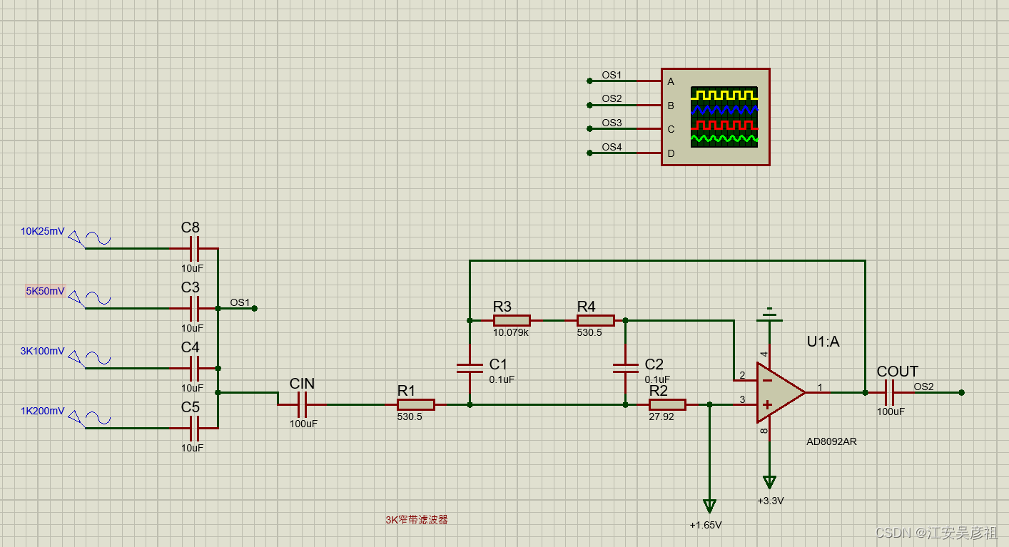
the simulation effect is as follows:
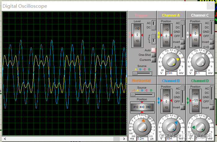
a horizontal grid is 0.2ms, and the filtered period is roughly 0.3ms, that is, 3KHZ.
TINA TI Simulation
Similarly, we also simulate on TINA TI:
the circuit diagram is as follows:

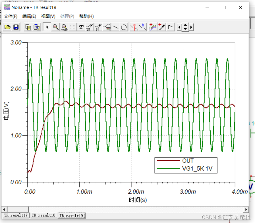
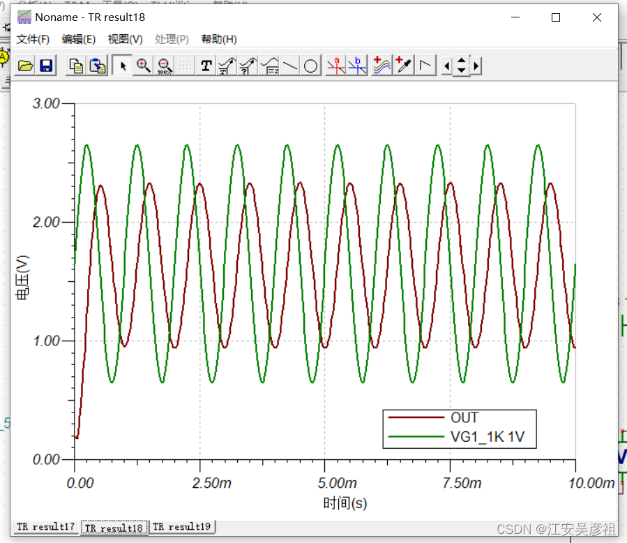
For a sinusoidal signal of 1K 0.1V, the response is as follows:
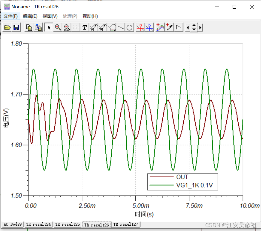
There is a slight amplification.
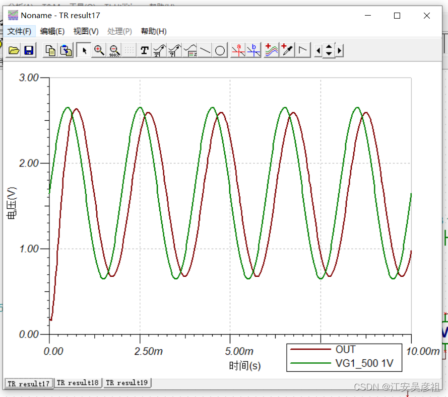
For a 3K signal, the response is as follows:
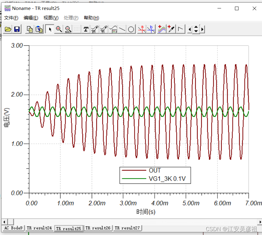
there is nearly a 10-fold amplification.
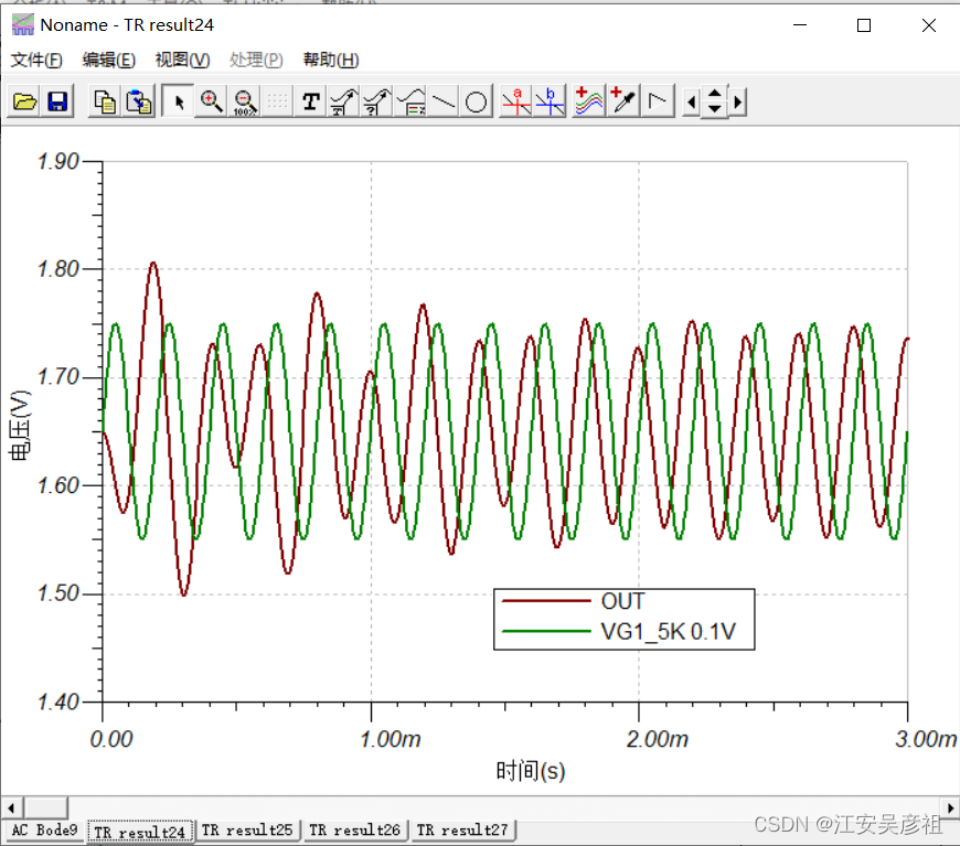
For 5K signals, the response is as follows: basically no amplification.
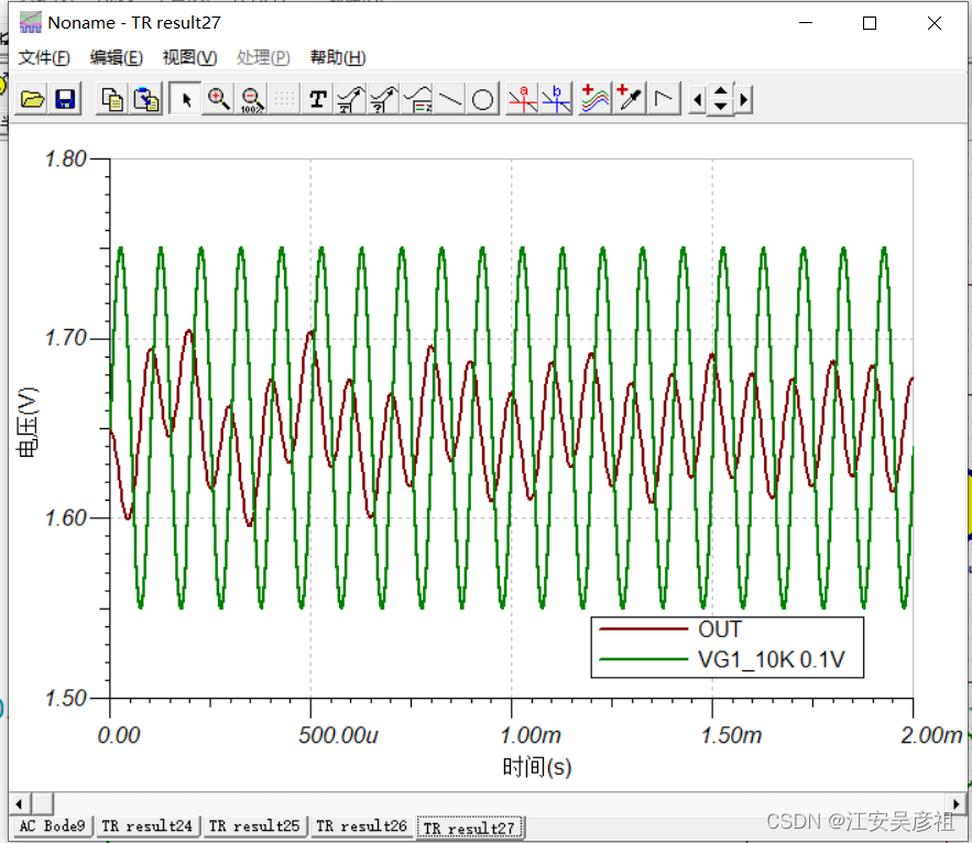
For a 10K signal, the response is as follows: basically no amplification.
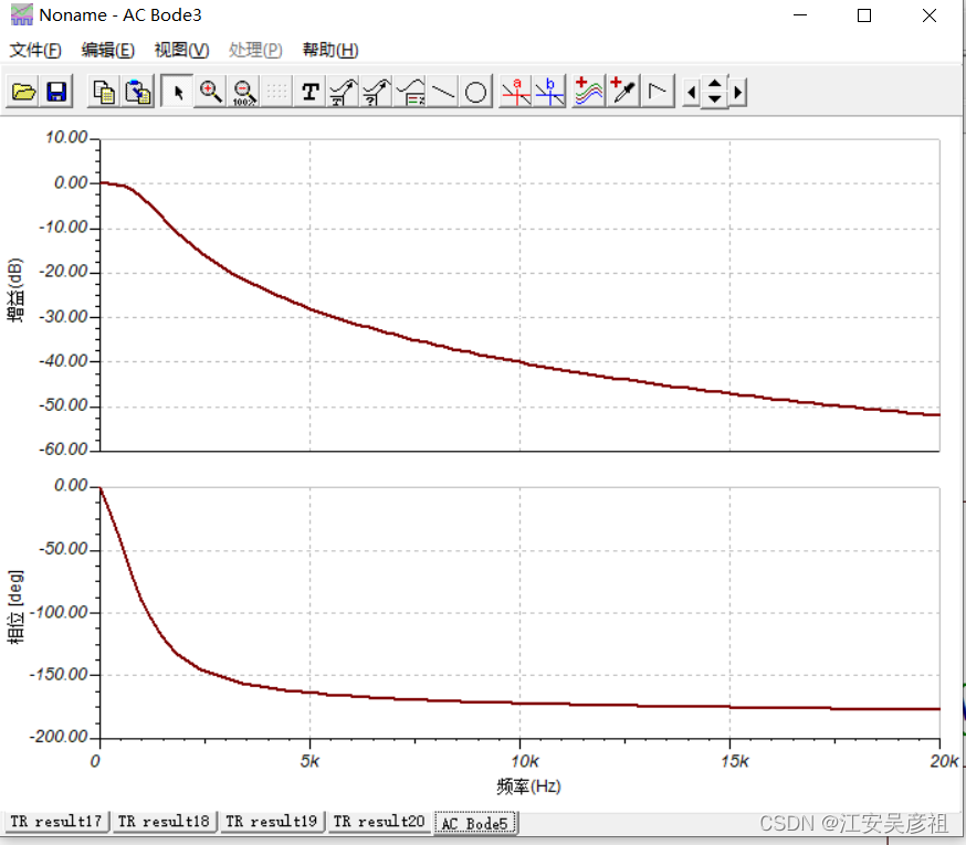
Look at its frequency characteristics, as follows:
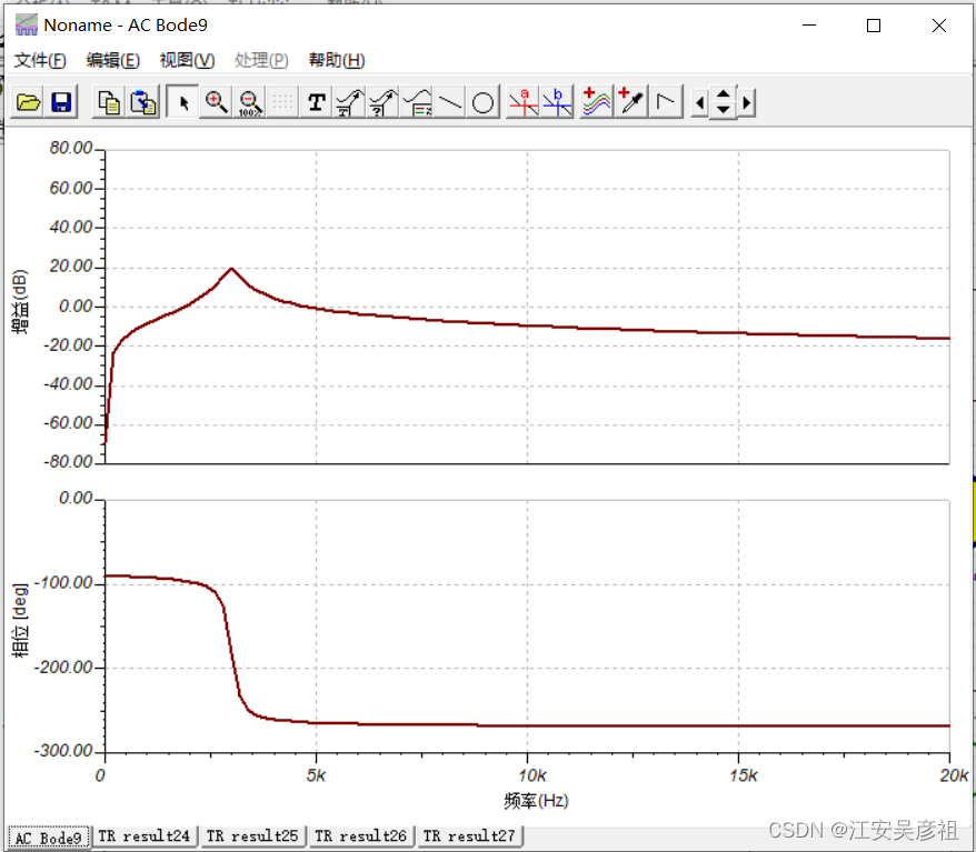
It is found that it has a good narrow-band filtering effect.
reference
Proteus amplifier simulation
Zhaogong
Tina TI
SPICE model
import model
TI official website design resources
include filters and other circuit design resources:
