↓Recommend attention↓

Hello everyone, among the various Python toolkits, Pandas should be the most frequently used. Today I will introduce to you various commonly used operations in Pandas in a graphical way. The content is a bit long. If you like it, remember to like, bookmark, and follow.

Part 1: Pandas Demonstration

Please see the table below:

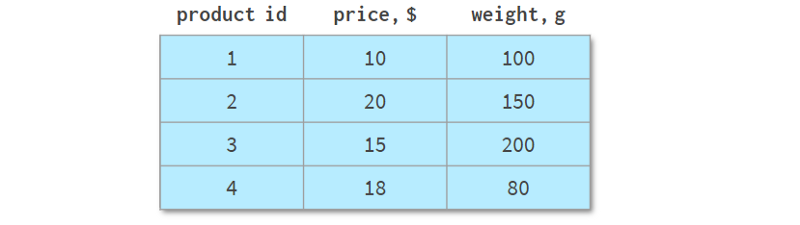
It describes the different product lines of an online store, with a total of four different products. Unlike the previous examples, it can be represented as a NumPy array or a Pandas DataFrame. But let's look at some of its common operations.

1. Sort

Sorting by column is more readable with Pandas, like so:

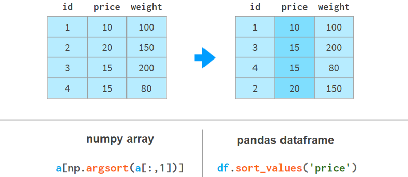
Here argsort(a[:,1]) computes the permutation that sorts the second column of a in ascending order, then a[…] reorders the rows of a accordingly. Pandas can do it in one step.

2. Sort by multiple columns

It gets even worse if we need to use the weight column to sort the price column. Here are a few examples to illustrate our point:

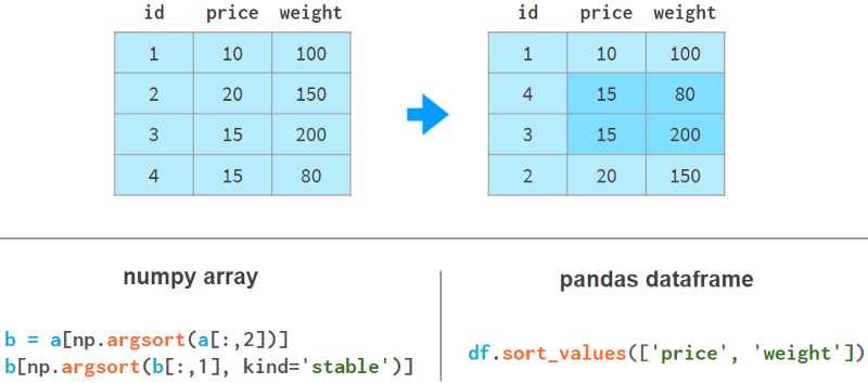
In NumPy, we sort by weight first and then by price. The stable sort algorithm guarantees that the results of the first sort will not be lost during the second sort. There are other implementations for NumPy, but none as simple and elegant as Pandas.

3. Add a column

Using Pandas to add columns is much nicer syntactically and architecturally. The following example shows how to do it:

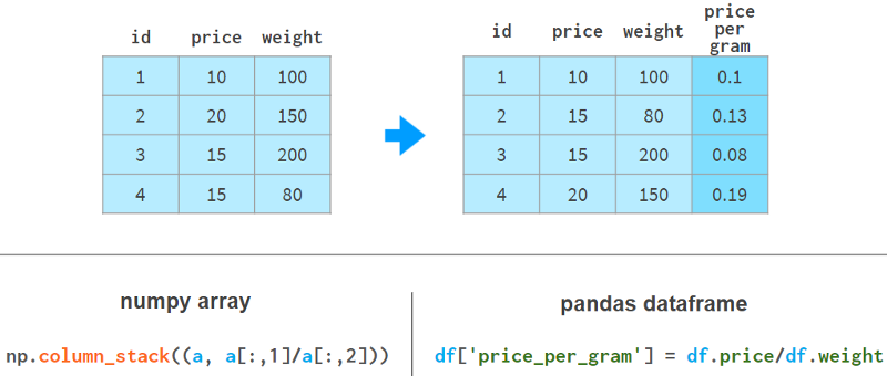
Pandas doesn't need to reallocate memory for the entire array like NumPy does; it just adds references to the new columns and updates the `registry` of column names.

4. Fast element search

In NumPy arrays, even if you're looking for the first element, you still need time proportional to the size of the array to look it up. With Pandas, you can index the columns you expect to be queried the most and reduce the search time to a constant.

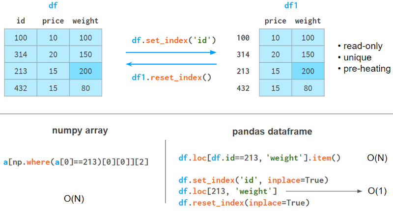
The index column has the following restrictions.

It takes memory and time to build.
It is read-only (needs to be rebuilt after each append or delete operation).
The values don't need to be unique, but the speedup will only happen if the elements are unique.
It needs to be warmed up: the first query is slightly slower than NumPy, but subsequent queries are significantly faster.

5. Join by column

If you want to get information based on the same column from another table, NumPy is hardly of any help. Pandas is better, especially for 1:n relationships.

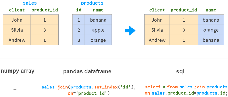
Pandas join has all the familiar "inner", "left", "right" and "full outer" join modes.

6. Group by column

Another common operation in data analysis is grouping by columns. For example, to get the total sales for each product, you could do this:

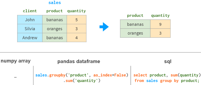
In addition to sum, Pandas also supports various aggregation functions: mean, max, min, count, etc.

7. PivotTable

One of the most powerful features of Pandas is the "pivot" table. It's a bit like projecting a multidimensional space onto a two-dimensional plane.

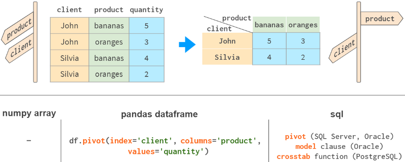
While it is certainly possible to do it with NumPy, this functionality is not available out of the box, although it is present in all major relational database and spreadsheet applications (Excel, WPS).

Pandas combines grouping and pivoting in one tool with df.pivot_table.

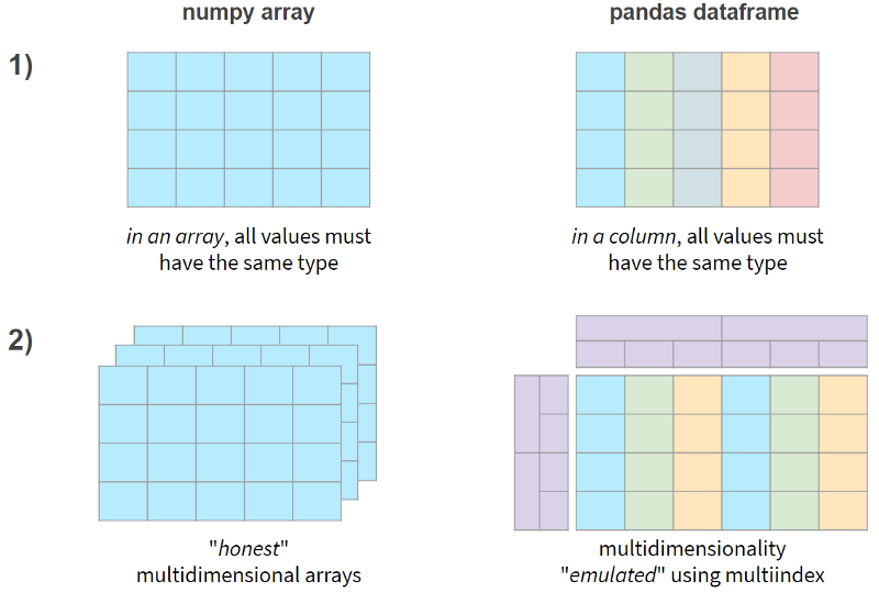
In short, the two main differences between NumPy and Pandas are as follows:

Now, let's see if these features come at a performance penalty.

8. Pandas speed

I benchmarked NumPy and Pandas on a typical Pandas workload: 5-100 columns, 10³-10⁸ rows, integers and floats. Here are the results for 1 row and 100 million rows:

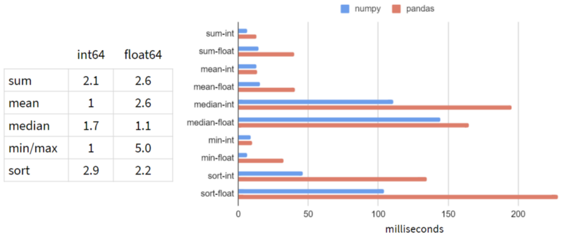
It looks like Pandas is slower than NumPy in every operation!

The situation doesn't change (predictably) when the number of columns increases. As for the number of rows, the dependencies (on a logarithmic scale) look like this:

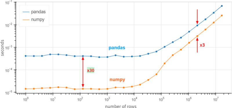
Pandas seems to be 30 times slower than NumPy for small arrays (less than 100 rows), and 3 times slower for large arrays (over 1 million rows).

How is that possible? Maybe it's time to submit a feature request suggesting that Pandas reimplement df.column.sum() via df.column.values.sum()? The values attribute here provides access to the underlying NumPy array, with performance improvements 3 ~ 30 times.

the answer is negative. Pandas is very slow at these basic operations because it handles missing values correctly. Pandas needs NaNs (not-a-number) to implement all these database-like mechanisms like grouping and pivoting, and that's common in the real world. In Pandas, we have done a lot of work to unify the use of NaN for all supported data types. By definition (enforced at the CPU level), nan+anything gets nan. so

>>> np.sum([1, np.nan, 2])  
nan

but

>>> pd.Series([1, np.nan, 2]).sum()  
3.0

A fair comparison would be to use np.nansum instead of np.sum, np.nanmean instead of np.mean, etc. suddenly……

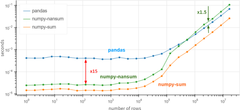
For arrays over 1 million elements, Pandas is 1.5 times faster than NumPy. It's still 15x slower than NumPy for smaller arrays, but generally it doesn't matter much whether the operation completes in 0.5 ms or 0.05 ms -- it's fast anyway.

On top of that, if you are 100% sure that there are no missing values in the column, you can get a x3-x30 performance boost by using df.column.values.sum() instead of df.column.sum(). In the presence of missing values, Pandas is quite fast and even outperforms NumPy for huge arrays (more than 10 homogeneous elements).

Part II. Series and Index

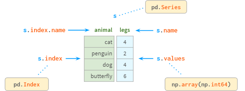
A Series is a one-dimensional array in NumPy and is the fundamental building block of a DataFrame representing its columns. Although its practical importance is diminishing compared to DataFrames (you can perfectly solve many practical problems without knowing what a Series is), it can be difficult to understand how DataFrames work without first learning about Series and Indexes. work.

Internally, Series stores values in plain NumPy vectors. Therefore, it inherits its advantages (compact memory layout, fast random access) and disadvantages (type homogeneity, slow deletion and insertion). Most importantly, Series allows its values to be accessed through labels using a dictionary-like structure index. Labels can be of any type (usually strings and timestamps). They don't have to be unique, but uniqueness is necessary to improve lookup speed, and many operations assume uniqueness.

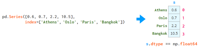
As you can see, each element can now be addressed in two alternative ways: by `label` (=with index) and by `position` (=without index):

Addressing by "location" is sometimes called "location indexing", which just adds to the confusion.

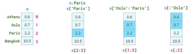
A pair of square brackets is not enough. in particular:

S[2:3] is not the most convenient way to resolve element 2
s[1:3] is ambiguous if the name happens to be an integer. It could mean that names 1 to 3 are inclusive or positional indices 1 to 3 are not.

To solve these problems, Pandas also has two "styles" of square brackets, which you can see below:

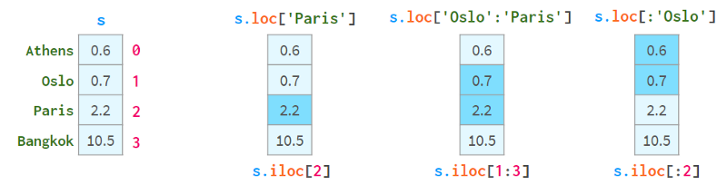
.loc always uses labels and includes both ends of the interval.

.iloc always uses the "position index" and excludes the right end.

The purpose of using square brackets instead of parentheses is to access Python's slicing convention: you can use single or double colons, which have the familiar start:stop:step meaning. As usual, the absence of start(end) means from the beginning of the sequence (to the end). The step parameter allows referencing even rows with s.iloc[::2] and getting elements in reverse order with s['Paris':'Oslo':-1] .

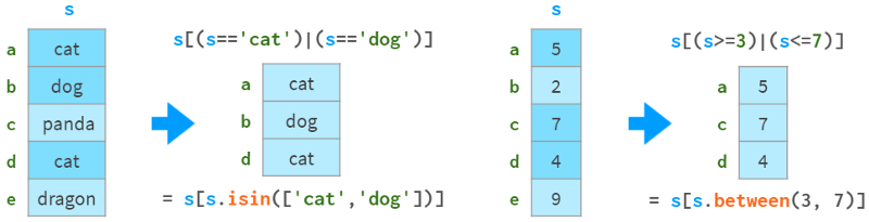
They also support boolean indexing (indexing with boolean arrays), as shown in the following image:

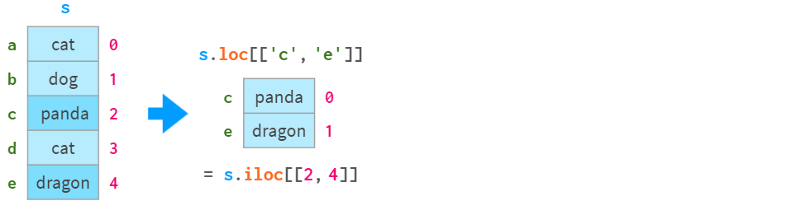
You can see how they support `fancy indexing` (indexing with integer arrays) in the image below:

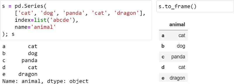
The worst thing about Series is its visual presentation: for some reason, it doesn't have a nice rich-text look, so it feels like a second-class citizen compared to DataFrame:

I patched the Series to make it look better, as follows:

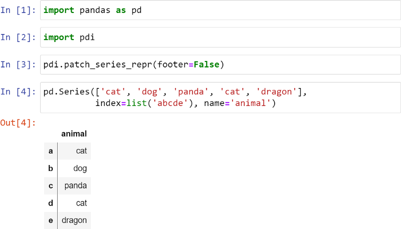
The vertical line indicates that this is a Series, not a DataFrame. Footer is disabled here, but it can be used to display dtypes, especially categorical types.

You can also display multiple Series or dataframes side by side using pdi.sidebyside(obj1, obj2, ...) :

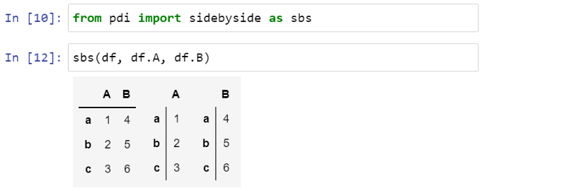
PDI (stands for pandas illustrated) is an open source library on github that has this and other functionality needed for this article. To use it, write

pip install pandas-illustrated

Index

The object responsible for getting elements by tags is called index. It's very fast: whether you have 5 rows or 5 billion rows, you can fetch a row of data in constant time.

The index is a true polymorphic creature. By default, when creating a Series (or DataFrame) without an index, it is initialized as a lazy object, similar to Python's range(). Like range, uses hardly any memory and is indistinguishable from positional indices. Let's create a sequence with one million elements using the following code:

>>> s = pd.Series(np.zeros(10**6))  
>>> s.index  
RangeIndex(start=0, stop=1000000, step=1)  
>>> s.index.memory_usage()       # in bytes  
128                    # the same as for Series([0.])

Now, if we remove an element, the index is implicitly converted to a dict-like structure, as follows:

>>> s.drop(1, inplace=True)  
>>> s.index  
Int64Index([     0,      2,      3,      4,      5,      6,      7,  
            ...  
            999993, 999994, 999995, 999996, 999997, 999998, 999999],  
           dtype='int64', length=999999)  
>>> s.index.memory_usage()  
7999992

This structure consumes 8Mb of memory! To get rid of it and go back to the lightweight range-like structure, add the following code:

>>> s.reset_index(drop=True, inplace=True)  
>>> s.index  
RangeIndex(start=0, stop=999999, step=1)  
>>> s.index.memory_usage()  
128

If you're not familiar with Pandas, you're probably wondering why Pandas doesn't do this itself? Well, for non-numeric labels, it's pretty obvious: why (and how) does Pandas, after deleting a row, relabel all subsequent rows ? For numeric labels, the answer is a bit more complicated.

First, as we've already seen, Pandas allows you to refer to rows purely by position, so if you want to target row 5 after deleting row 3, you can do so without reindexing (that's what iloc does).

Second, keeping the original tab is a way to keep in touch with moments from the past, much like a "save game" button. Suppose you have a large table of 100x1000000 and need to look up some data. You're doing several queries one after another, narrowing the search each time, but only looking at a small set of columns, because it's impractical to look at hundreds of fields at the same time. Now that you have found the rows of interest, you want to see all the information about them in the original table. Digital Index helps you get it right away without any extra effort.

In general, it's a good idea to keep values unique within an index. For example, lookup speed is not improved when there are duplicate values in the index. Pandas doesn't have "unique constraints" like relational databases (the feature is still experimental), but it has functions to check if values in an index are unique, and to eliminate duplicates in various ways.

Sometimes one column is not enough to uniquely identify a row. For example, cities with the same name sometimes happen to be in different countries, or even different parts of the same country. So (city, state) is a better candidate than city to identify a place. In databases, this is called a "composite primary key". In Pandas, it's called a multi-index (see section 4 below), and each column in the index is called a "level".

Another important property of indexes is immutability. Unlike a normal column in a DataFrame, you cannot change it in-place. Any change in an index involves fetching data from the old index, modifying it, and reattaching the new data as the new index. Usually, it's transparent, which is why you can't just write df.City.name = ' city ', but you have to write a less obvious df.rename(columns={'A': 'A'}, inplace =True)

Index has a name (in case of MultiIndex, each level has a name). Unfortunately, this name is underused in Pandas. Once you include this column in your index, you can't use df anymore. Column name notation is no longer used and has to revert to less readable df. Index or the more general df. loc For multi-index, the situation is even worse. A notable exception is df. Merge - You can specify the column to merge by name, whether it is in the index or not.

The same indexing mechanism is used to label dataframe rows and columns, as well as sequences.

Find element by value

A Series internally consists of a NumPy array and an array-like structure index, as follows:

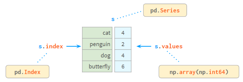
Index provides a convenient way to look up values by label. So how do you lookup tags by value?

s.index[s.tolist().find(x)]           # faster for len(s) < 1000  
s.index[np.where(s.values==x)[0][0]]  # faster for len(s) > 1000

I wrote two simple wrappers for find() and findall() that are fast (because they automatically choose the actual command based on the size of the sequence) and are more convenient to use. The code looks like this:

>>> import pdi  
>>> pdi.find(s, 2)  
'penguin'  
>>> pdi.findall(s, 4)  
Index(['cat', 'dog'], dtype='object')

missing value

Pandas developers pay special attention to missing values. Normally, you receive a dataframe with NaNs by providing a flag to read_csv. Otherwise, None can be used in the constructor or assignment operator (although the implementation of different data types is slightly different, it still works). This image helps explain the concept:

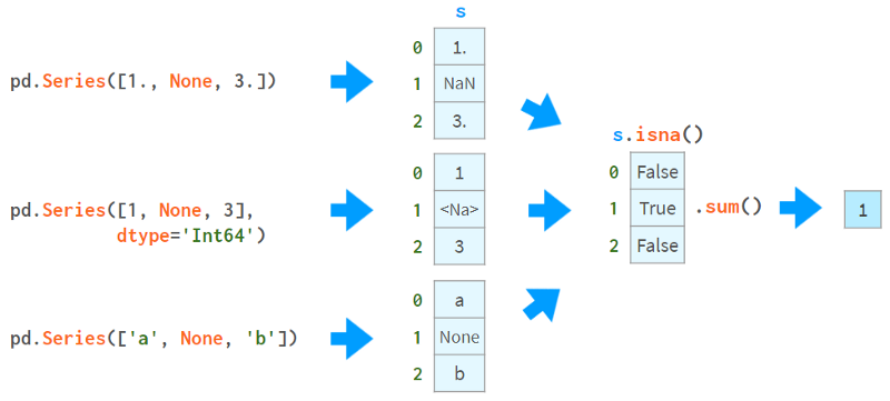
The first thing you can do with NaNs is find out if you have NaNs. As you can see from the image above, isna() produces a boolean array, while .sum() gives the total number of missing values.

Now that you know they exist, you can choose to fill them with constant values or remove them all at once through interpolation, like so:

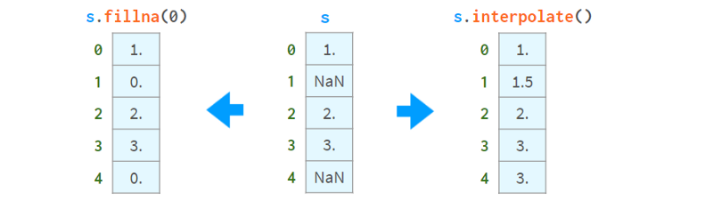
On the other hand, you can keep using them. Most Pandas functions will happily ignore missing values, as shown in the image below:

More advanced functions (median, rank, quantile, etc.) can do this too.

Arithmetic operations are aligned with indices:

Inconsistent results if there are non-unique values in the index. Do not use arithmetic operations on sequences whose indices are not unique.

Compare

Comparing arrays with missing values can be tricky. Below is an example:

>>> np.all(pd.Series([1., None, 3.]) ==   
           pd.Series([1., None, 3.]))  
False  
>>> np.all(pd.Series([1, None, 3], dtype='Int64') ==   
           pd.Series([1, None, 3], dtype='Int64'))  
True  
>>> np.all(pd.Series(['a', None, 'c']) ==   
           pd.Series(['a', None, 'c']))  
False

To compare nans correctly, you need to replace nans with elements that must not be in the array. For example, using -1 or ∞:

>>> np.all(s1.fillna(np.inf) == s2.fillna(np.inf))   # works for all dtypes  
True

Or, better yet, use NumPy or Pandas' standard comparison functions:

>>> s = pd.Series([1., None, 3.])  
>>> np.array_equal(s.values, s.values, equal_nan=True)  
True  
>>> len(s.compare(s)) == 0  
True

Here, the compare function returns a list of differences (actually a DataFrame), and array_equal returns a boolean directly.

NumPy comparisons fail when comparing DataFrames of mixed types (issue #19205), whereas Pandas works just fine. As follows:

>>> df = pd.DataFrame({'a': [1., None, 3.], 'b': ['x', None, 'z']})  
>>> np.array_equal(df.values, df.values, equal_nan=True)  
TypeError  
<...>  
>>> len(df.compare(df)) == 0  
True

append, insert, delete

Although a Series object is considered immutable in size, it can append, insert, and delete elements in-place, but all of these operations are:

Slow because they require reallocating memory and updating indexes for the entire object.
very inconvenient.

Here's one way to insert a value and two ways to delete a value:

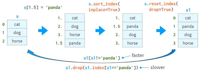
The second method of removing values (via drop) is slower and can lead to complex bugs when there are non-unique values in the index.

Pandas has the df.insert method, but it can only insert columns (not rows) into a dataframe (and doesn't work on series).

Another way to add and insert is to slice the DataFrame using iloc, apply the necessary transformations, and then use concat to put it back. I implemented a function called insert that automates this process:

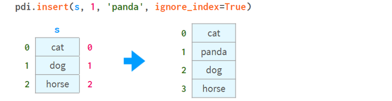
Note that (as in df.insert ) the insertion position is specified by position 0 <= i <= len(s), not the label of the element in index. As follows:

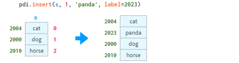
To insert by element's name, you can combine pdi. Find it with pdi. Insert, as follows:

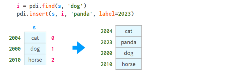
Note that unlikedf.insert, pdi.insert return a copy instead of modifying the Series/DataFrame in-place

Statistical data

Pandas provides a full range of statistical functions. They allow you to understand what's in a million-element sequence or DataFrame without manually scrolling through the data.

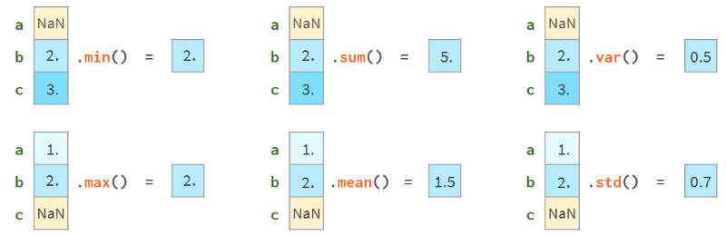
All Pandas statistical functions ignore NaNs, as follows:

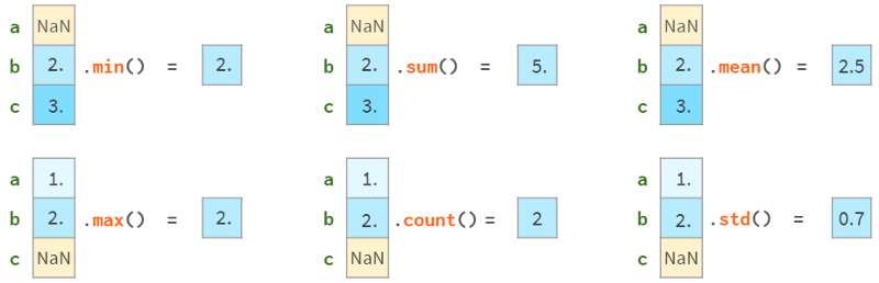
Note that Pandas std gives different results than NumPy std, as follows:

>>> pd.Series([1, 2]).std()  
0.7071067811865476  
>>> pd.Series([1, 2]).values.std()  
0.5

This is because NumPy std uses N as the denominator by default, while Pandas std uses N-1 as the denominator by default. Both stds have a parameter called ddof (`delta degrees of freedom`), which defaults to 0 for NumPy and 1 for Pandas, which can make the results consistent. N-1 is what you usually want (to estimate the bias of a sample when the mean is unknown). Here's a wikipedia article detailing Bezier's correction.

Since each element in a sequence can be accessed by label or position index, argmin (argmax) has a sister function idxmin (idxmax), as shown in the following figure:

Here are Pandas' self-describing statistical functions for reference:

std: sample standard deviation
var, unbiased variance
sem, unbiased standard error of the mean
quantile quantile, main quantile(s.quantile(0.5)≈s.median())
oode is the most frequently occurring value
Defaults to Nlargest and nsmallest, in order of appearance
diff, the first discrete difference
cumsum 和 cumprod、cumulative sum和product
cummin and cummax, cumulative minimum and maximum values

and some more specialized statistical functions:

pct_change, the percentage change between the current element and the previous element
skew skewed state, unbiased state (third-order moment)
kurt or kurtosis, unbiased kurtosis (fourth moment)
cov, corr and autocorr, covariance, correlation and autocorrelation
rolling rolling window, weighted window and exponentially weighted window

Duplicate data

Special care needs to be taken when detecting and handling duplicate data, as shown in the following diagram:

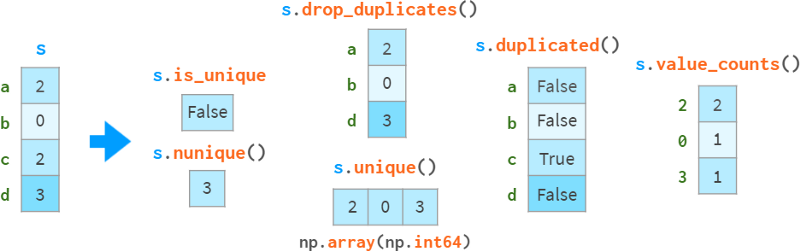
drop_duplicates and duplication can keep the last occurrence of the duplicate instead of the first occurrence.

Note that sa uint() is faster than np. Uniqueness (O(N) vs O(NlogN)), it preserves order and doesn't return sorted results. Unique.

Missing values are treated as ordinary values, which can sometimes lead to surprising results.

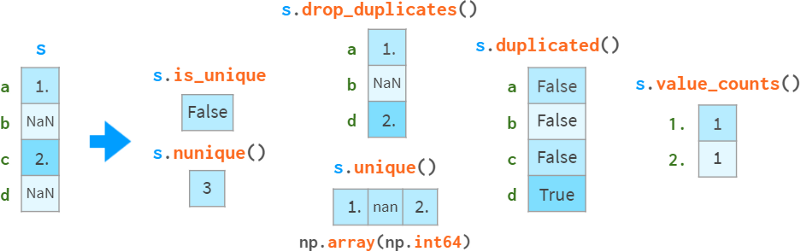
If you want to exclude nan, you need to do so explicitly. In this example, sl opdropna().is_unique == True.

There is also a class of monotonic functions whose names are self-describing:

s.is_monotonic_increasing ()
s.is_monotonic_decreasing ()
s._strict_monotonic_increasing ()
s._string_monotonic_decreasing ()
s. is_monotonic(). This is unexpected, for some reason this is s.is_monotonic_increasing(). It only returns False for monotonically decreasing sequences.

group

In data processing, a common operation is to compute some statistics, not for the entire data set, but for some groups within it. The first step is to define a "smart object" by providing criteria for decomposing a series (or a dataframe) into groups. This `smart object` has no immediate representation, but it can be queried like a Series to get a certain property of each group, as shown in the image below:

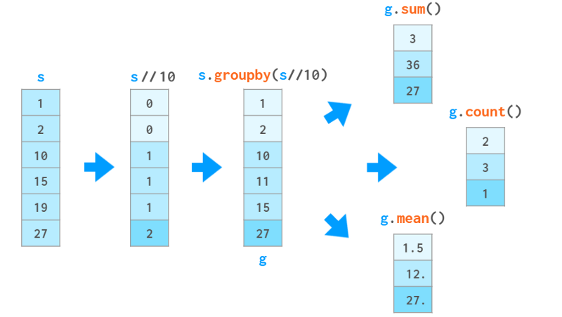
In this example, we divide the sequence into three groups based on the integer part of the value divided by 10. For each group, we request the sum of the elements in each group, the number of elements, and the average.

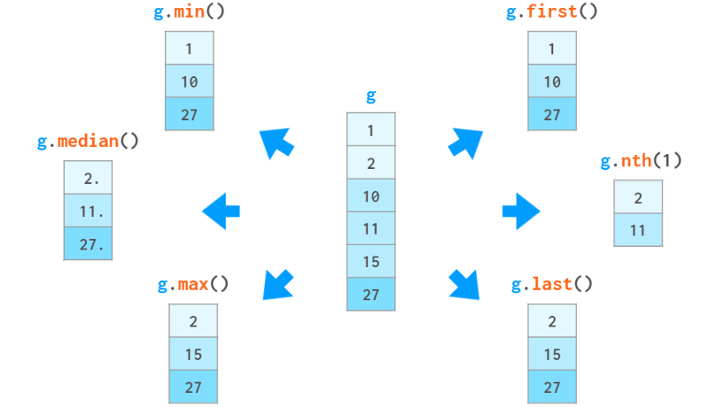
In addition to these aggregate functions, you can also access specific elements based on their position within the group or their relative value. As follows:

You can also use g.ag(['min', 'max']) to evaluate multiple functions in one call, or use gc describe() to display a bunch of statistical functions at once.

And if that's not enough, you can also pass data through your own Python functions. it can be:

A function f that takes a group x (a Series object) and produces a value (such as sum() ) for use with g.eapply(f).

A function f that takes a group x (a Series object) and with g.transform(f) produces a Series object of the same size as x (eg cumsum() ).

In the above example, the input data is ordered. groupby doesn't need to do this. In fact, it works just as well if the elements in the grouping are not stored contiguously, so it's closer to collections.defaultdict than to itertools.groupby. It always returns an index with no duplicates.

Unlike defaultdict and the relational database GROUP BY clause, Pandas groupby sorts the results by group name. It can be disabled with sort=False.

Disclaimer: Actually, g.apply(f) is more general than described above:

If f(x) returns a sequence of the same size as x, it can simulate transform
If f(x) returns a sequence of differently sized or distinct dataframes, you get a sequence with a corresponding multiindex.

But the documentation warns that using these methods may be slower than the corresponding transform and agg methods, so be careful.

Part 3. DataFrames

The main data structure of Pandas is DataFrame. It bundles a two-dimensional array with labels for its rows and columns. It consists of a sequence of objects (with a shared index), each object representing a column, possibly of a different dtype.

Read and write CSV files

A common way to construct a DataFrame is to read a csv (comma-separated values) file, as shown in the image below:

The pd.read_csv() function is a fully automated and wildly customizable tool. If you only want to learn one thing about Pandas, learn to use read_csv - it will pay off :).

Here is an example of parsing a non-standard .csv file:

and some brief descriptions:

Because CSV doesn't have a strict specification, it sometimes takes a bit of trial and error to read it correctly. The cool thing about read_csv is that it automatically detects a lot of things:

column names and types
Representation of boolean values
Representation of missing values, etc.

As with any automation, you better make sure it's doing the right thing. If the result of simply writing df in a Jupyter cell happens to be too long (or too incomplete), you can try the following:

df.head(5) or df[:5] displays the first 5 rows
df.dtypes returns the types of the columns
df.shape returns the number of rows and columns
Df.info() summarizes all relevant information

It is a good idea to set one or several columns as indexes. The diagram below illustrates this process:

Index has many uses in Pandas:

Arithmetic operations are aligned by index
It makes lookups by that column faster, etc.

All this comes at the cost of higher memory consumption and less obvious syntax.

Build DataFrame

Another option is to build a dataframe from data already stored in memory. Its constructor is very versatile and can convert (or wrap) any type of data:

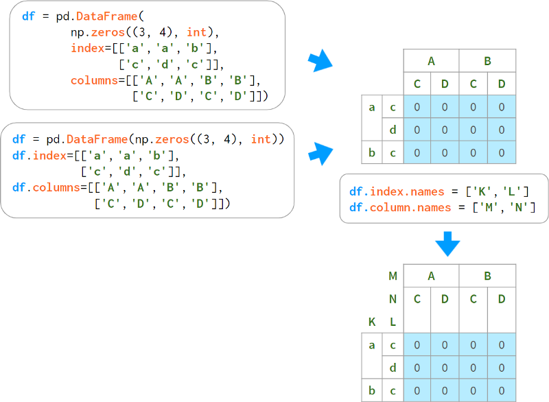
In the first case, in the absence of row labels, Pandas labels rows with consecutive integers. In the second case it does the same for both rows and columns. It's always a good idea to provide Pandas with the names of columns instead of integer labels (using the columns argument), and sometimes rows (using the index argument, although rows might sound more intuitive). This picture will help:

Unfortunately, there is no way to set a name for an index column in the DataFrame constructor, so the only option is to specify it manually, e.g., df.index.name = 'cityname'

The next approach is to construct a DataFrame from a dictionary of NumPy vectors or a two-dimensional NumPy array:

Note that in the second case, the value of the population size is converted to a floating point number. In fact, it happened before when building NumPy arrays. Another thing to note here is that building a dataframe from a 2D NumPy array is a view by default. This means changing the values in the original array will change the dataframe and vice versa. Plus, it saves memory.

The first case (a dictionary composed of NumPy vectors) can also enable this mode, just set copy=False. However, it is very fragile. A simple operation can turn it into a replica without notification.

Two other (less useful) options for creating a DataFrame are:

From a list of dicts (where each dict represents a row whose keys are column names and whose values are corresponding cell values)
From a dict of Series (where each Series represents a column; it can be made to return a view with copy=False by default).

If you register stream data "on the fly", your best bet is to use a dict of lists or a list of lists, since Python will transparently preallocate space at the end of the list for fast appending. Neither NumPy arrays nor Pandas dataframes can do this. Another possibility (if you know the number of rows in advance) is to manually pre-allocate the memory with something like DataFrame(np.zeros).

Basic operations on DataFrames

The best thing about DataFrames (in my opinion) is that you can:

Easily access its columns, as d.area returns column values (or df[' Area '] - for column names containing spaces)
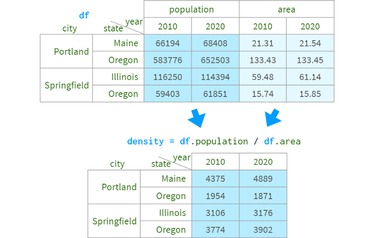
Manipulating columns as arguments, e.g. using afterdf.population /= 10**6 to store population in millions, the command below creates a new column called `density` based on the values in an existing column. See the image below for more information:

Note that when creating a new column, square brackets must be used even if the column name does not contain spaces.

Additionally, you can use arithmetic operations on columns in different dataframes as long as their rows have meaningful labels, like so:

Indexed DataFrames

As we've seen in this series, plain square brackets are not enough for all the needs of indexing. You can't access rows by name, you can't access disjoint rows by positional index, and you can't even refer to individual cells, because df['x', 'y'] is reserved for multi-indexing!

To meet these needs, dataframes, like series, have two optional indexing modes: loc by label and iloc by position.

In Pandas, referencing multiple rows/columns is a copy, not a view. But it's a special kind of copy that allows assignment as a whole:

df.loc['a']=10 works (a line as a whole is a writable)
df.loc['a']['A']=10 works (element access propagated to original df)
df.loc['a':'b'] = 10 works (assigning to a subar assigns the entire work to a subarray)
df.loc['a':'b']['A'] = 10 doesn't (assigning to its elements doesn't).

In the last case, the value will only be set on the copy of the slice and not reflected on the original df (a warning will be displayed accordingly).

Depending on the context, there are different solutions:

You want to alter the original df. Then use df. loc['a': 'b', 'a'] = 10
You intentionally created a copy and then want to dispose of this copy: df1 = df.loc[' a ': ' b '];df1[' A ']=10 # SettingWithCopy warning To suppress the warning in this case, please Make it a true copy: df1 = df.loc[' A ': ' b '].copy(); df1[A] = 10

Pandas also supports a convenient NumPy syntax for boolean indexing.

When using multiple conditions, they must be enclosed, like this:

Special care is required when you expect a value to be returned.

Because there may be multiple rows matching the condition, loc returns a sequence. To get a scalar value from it, you can use:

float(s), or more generally se item(), will raise ValueError unless there is only one value in the sequence

S.iloc[0] , only throws an exception if not found; moreover, it's the only function that supports assignment: df[…].Iloc[0] = 100 , but you definitely don't need it when you want to modify all matches :df[…]=100.

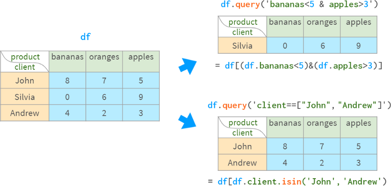
Alternatively, you can use string-based queries:

df.query (' name = =“Vienna”)

df.query('population>1e6 and area<1000') they are shorter, suitable for multi-indexing, and logical operators are preferred over comparison operators (= less parentheses required), but they can only filter by row, and cannot Modify Dataframe by them.

Several third-party libraries allow you to query dataframes directly using SQL syntax (duckdb), or indirectly by copying the dataframe to SQLite and wrapping the results back into Pandas objects (pandasql). As expected, the direct method is faster.

DataFrame arithmetic

You can apply common operations on dataframes, series, and their combinations, such as addition, subtraction, multiplication, division, modulo, power, etc.

All arithmetic operations are aligned in terms of row and column labels:

In a hybrid operation between a dataframe and a Series, the Series (god knows why) behaves (and broadcasts) like a row vector, and aligns accordingly:

Possibly for consistency with lists and 1D NumPy vectors (they are not aligned by labels and are considered a simple DataFrame of 2D NumPy arrays):

So, in the less fortunate (and most common!) case of dividing a dataframe by a sequence of column vectors, you have to use methods instead of operators, like so:

Because of this questionable decision, whenever you need to perform a mixed operation between a dataframe and a columnar sequence, you have to look it up (or memorize it) in the documentation:

Combining DataFrames

Pandas has three functions, concat, merge, and join, that do the same thing: combine information from multiple dataframes into one. But each tool implements it slightly differently, as they are tailored for different use cases.

vertical stack

This is probably the easiest way to combine two or more dataframes into one: you take the rows from the first dataframe and append the rows from the second dataframe to the bottom. For this to work, the two dataframes need to have (roughly) the same columns. This is similar to vstack in NumPy, as you can see in the image:

It is not good to have duplicate values in the index. You may run into all sorts of problems (see `drop` examples below). Even if you don't care about indexes, try to avoid duplicate values:

Either use the reset_index=True parameter
call df.reset_index(drop=True) to reindex rows from 0 to len(df)-1,
The ambiguity of MultiIndex can be resolved using the keys parameter (see below).

If the columns of the dataframe don't match perfectly (different orders don't count here), Pandas can take the intersection of the columns (default kind='inner') or insert nan to mark missing values (kind='outer'):

horizontal overlay

concat can also perform "horizontal" stacking (similar to hstack in NumPy):

join is more configurable than concat: in particular, it has five join modes, while concat has only two. See the "1:1 Relationship Connections" section below for details.

Multi-index based data overlay

concat can perform multi-indexing similar to vertical stacking (like dstack in NumPy) if the row and column labels coincide:

If the rows and/or columns partially overlap, Pandas will align the names accordingly, which is most likely not what you want. The diagram below can help you visualize this process:

In general, if labels overlap, it means that the dataframes are somehow related to each other, and the relationship between entities is best described using relational database terms.

1:1 connected relationship

When information about the same set of objects is stored in several different DataFrames, you want to merge them into one DataFrame.

Use merge if the columns to be merged are not in the index.

The first thing it does is discard whatever is in the index. Then perform the join operation. Finally, renumber the result from 0 to n-1.

If the column is already in the index, you can use join (this is just an alias for merge, with left_index or right_index set to True, and a different default).

As you can see from this simplified example (see full outer join above), Pandas handles row order quite lightly compared to relational databases. Left and right outer joins are more predictable than inner and outer joins (at least until there are duplicate values in the columns that need to be merged). Therefore, if you want to guarantee row order, you must explicitly sort the results.

1:n connection relationship

This is the most widely used relationship in database design. A row in table A (such as "State") can be related to several rows in table B (such as cities), but each row in table B can only be related to a row in table A. (i.e. a city can only be in one state, but a state consists of multiple cities).

Just like with 1:1 relationships, to join a pair of 1:n related tables in Pandas, you have two options. Use merge if the columns to be merged are either not in the index and you can discard columns that happen to be in the indexes for both tables. The following example will help:

As we've seen, merge is less strict about row order than Postgres: for all declared statements, key order is preserved only when left_index=True and/or right_index=True (which is an alias for join ), and only when When there are no duplicate values in the merged column. That's why join has a sort parameter.

Now, if the columns to be merged are already in the right DataFrame's index, you can use join (or merge with right_index=True, which is the exact same thing):

This time Pandas preserves the index values and row order of the left DataFrame.

NOTE: Note that if the second table has duplicate index values, you will end up with duplicate index values in the result, even if the left table index is unique!

Sometimes, the merged dataframe has columns with the same name. Both merge and join have methods to resolve ambiguity, but the syntax is slightly different (by default, merge will use `_x`, `_y` to resolve, while join will throw an exception), as shown in the following figure:

Summarize:

Merge joins on non-indexed columns that require columns to be indexed
merge discards the index of the left DataFrame, join keeps it
By default, merge performs an inner join and join performs a left outer join
Merge does not preserve row order
Join can keep them (with some restrictions)
join is an alias for merge with left_index=True and/or right_index=True

multiple connections

As mentioned above, it acts as an alias for merge when running join on two dataframes such as df.join(df1) . But join also has a `multiple join` mode, which is just an alias for concat(axis=1).

Compared with normal mode, this mode has some limitations:

It doesn't provide a way to resolve duplicate columns
It only works for 1:1 relationships (index-to-index joins).

Therefore, multiple 1:n relationships should be connected one after the other. The repository `panda-illustrated` also provides a helper method as follows:

pdi.join is a simple wrapper around Join that accepts on, how and postfix arguments so you can do multiple joins in one command. As with the original join operation, the join is performed on the columns belonging to the first DataFrame, and the other DataFrames are joined according to their indices.

insert and delete

Since a DataFrame is a collection of columns, it is easier to apply these operations to rows than to columns. For example, inserting a column is always done in-place, while inserting a row always produces a new DataFrame as follows:

Dropping columns is generally nothing to worry about, except for del df['D'] and del df . D does not (Python-level restrictions).

Deleting rows using drop is very slow and can lead to complex bugs if the original tags are not unique. The following diagram will help explain the concept:

One solution is to use ignore_index=True, which tells concat to reset row names after concatenation:

In this case, setting the name column as an index will help. But for more complex filters, it won't.

Another solution that is fast, general, and even handles duplicate row names is to index instead of delete. To avoid explicitly negating the condition, I wrote an automated program (one line of code).

group

This operation has been described in detail in the Series section. But DataFrame's groupby has some specific tricks on top of that.

First, you can use a name to specify the column to group by, as shown in the following image:

Without as_index=False, Pandas specifies the grouping column as the index. If this is not what we want, we can use reset_index() or specify as_index=False.

Often, there are more columns in the data frame than you want to see in the result. By default, Pandas will sum everything that is remotely summable, so you'll need to narrow down your selection, like this:

Note that when summing a single column, you will get a Series instead of a DataFrame. If for some reason you want a DataFrame, you can:

Use double brackets: df.groupby('product')[['quantity']].sum()
Explicit conversion: df.groupby('product')['quantity'].sum().to_frame()

Switching to numeric indexing also creates a DataFrame:

df.groupby('product', as_index=False)['quantity'].sum()
df.groupby('product')['quantity'].sum().reset_index()

However, despite its unusual appearance, Series behaves just like DataFrames, so perhaps a "facelift" to pdi.patch_series_repr() is enough.

Obviously different columns behave differently when grouped. For example, summing quantities is perfectly fine, but summing prices doesn't make sense. use. Agg can specify different aggregation functions for different columns, as shown in the following figure:

Alternatively, you can create multiple aggregate functions for a column:

Or, to avoid tedious column renaming, you can do this:

Sometimes, the predefined functions are not enough to produce the desired result. For example, it would be better to use weights when averaging prices. You can provide a custom function for this. Unlike Series, this function can access multiple columns in a group (it takes a subdataframe as an argument), as follows:

Unfortunately, you can't combine predefined aggregations with several column-level custom functions, like the one above, because agg only accepts a single column-level user function. The only thing a user function with a single-column scope can access is the index, which is convenient in some cases. For example, bananas were on sale that day for 50% off, as shown in the image below:

In order to access the value of the group by column from the custom function, it has been included in the index beforehand.

Typically, the function with the least customization yields the best performance. For speed:

Implementing custom functions for multi-column ranges through g.apply()
Implement a custom function for a single-column range through g.agg() (supports acceleration using Cython or Numba)
A predefined function (Pandas or NumPy function object, or its string name).
A predefined function (Pandas or NumPy function object, or its string name).

A pivot table is a useful tool, often used with grouping, to view data from different perspectives.

Rotation and `Unrotation`

Suppose you have a variable a which depends on two parameters i and j. There are two equivalent ways to represent it as a table:

When the data is "dense" (when there are few 0 elements), the `short` format is more appropriate, and when the data is "sparse" (most elements are 0 and can be omitted from the table), the `long` format is more appropriate. `The format is better. Things get more complicated when there are more than two parameters.

Of course, there should be an easy way to convert these formats. Pandas provides a simple and convenient solution for this: pivot tables.

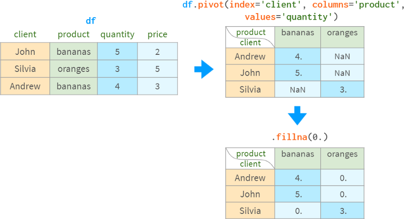
As a less abstract example, consider the sales data in the following table. There are two customers who purchased the specified quantities of two products. Initially, this data is in the short form. ` To convert it to `long format`, use df.pivot:

The command discards any information not relevant to the operation (index, price) and converts the information from the three requested columns to long form, putting the customer name in the index of the result, the product name in the column, and the sales Quantities are put into the `body` of the DataFrame.

For the opposite operation, you can use stack. It combines indexes and columns into a MultiIndex:

Another option is to use melt:

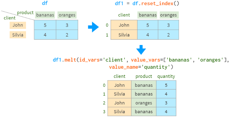
Note that melt sorts the result rows differently.

Pivot loses the name information of the `body` of the result, so whether it is stack or melt, we have to remind pandas of the name of the `quantity` column.

In the example above, all values are present, but this is not required:

The practice of grouping values and then pivoting the results is so common that groupby and pivot are bundled into a dedicated function (and corresponding DataFrame method) for pivot tables:

Without the columns argument, it behaves like groupby
It works similar to pivot when there are no duplicate rows to group by
Otherwise, it does the grouping and rotation

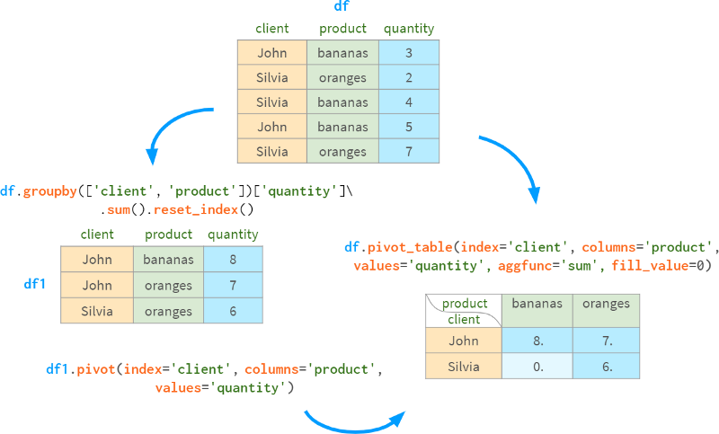
The aggfunc parameter controls which aggregate function should be used to group rows (default is mean).

For convenience, pivot_table can calculate subtotals and totals:

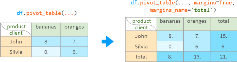
Once created, the pivot table becomes an ordinary DataFrame, so it can be queried using the standard methods described earlier.

Pivot tables are especially handy when using multiple indexes. We have seen many examples of Pandas functions returning multi-indexed DataFrames. Let's take a closer look.

Part IV. MultiIndex

For those who have never heard of Pandas, the most straightforward use of a MultiIndex is to use a second index column that complements the first to uniquely identify each row. For example, to disambiguate cities from different states, the name of the state is usually appended to the name of the city. For example, there are about 40 springfields in the US (in relational databases, it's called a composite primary key).

You can specify the columns to include in the index after parsing the DataFrame from CSV, or immediately as arguments to read_csv.

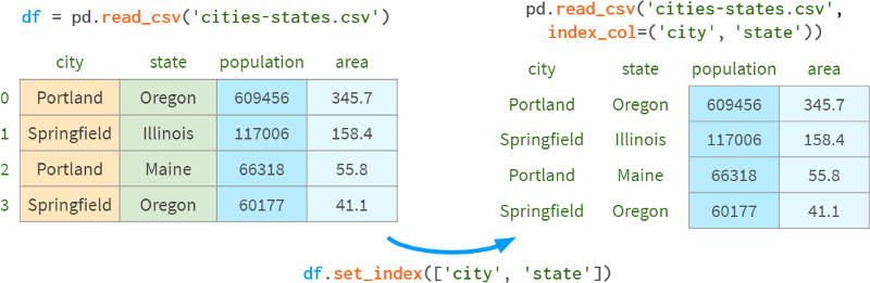
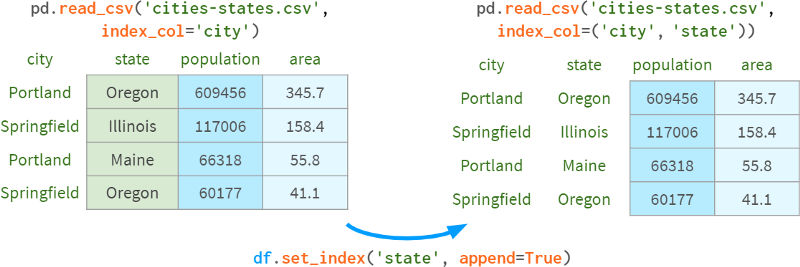
You can also add existing levels to a multiindex with append=True, as shown in the following image:

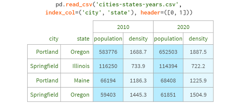
Another more typical use case is representing multiple dimensions. When you have a set of objects with specific properties or objects that evolve over time. For example:

Results of Sociological Survey
`Titanic` dataset
Historical Weather Observations
Chronology of Championship Rankings.

This is also known as "panel data", after which Pandas is named.

Let's add such a dimension:

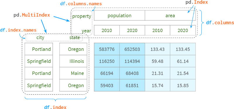
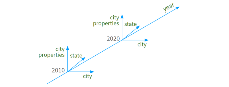
We now have a 4D space that looks like this:

Years form a (nearly continuous) dimension
City names are arranged along the second line
third state name
Specific urban attributes ("population", "density", "area", etc.) act as "tick marks" on the fourth dimension.

The following diagram illustrates the concept:

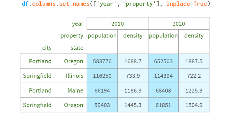
To make room for the dimension names of the corresponding columns, Pandas moves the entire header up:

group

The first thing to notice about a multiindex is that it doesn't group anything by the way it might appear. Internally, it's just a flattened sequence of tags, like this:

You can get the same groupby effect by sorting the row labels:

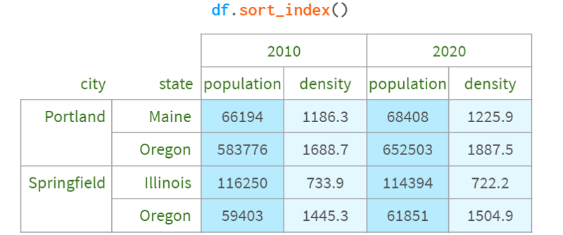
You can even disable visual grouping entirely by setting the corresponding Pandas option
: pd.options.display.multi_sparse=False .

type conversion

Pandas (and Python itself) distinguish between numbers and strings, so it's usually best to convert numbers to strings when the data type cannot be detected automatically:

pdi.set_level(df.columns, 0, pdi.get_level(df.columns, 0).astype('int'))

If you're feeling adventurous, you can do the same with standard tools:

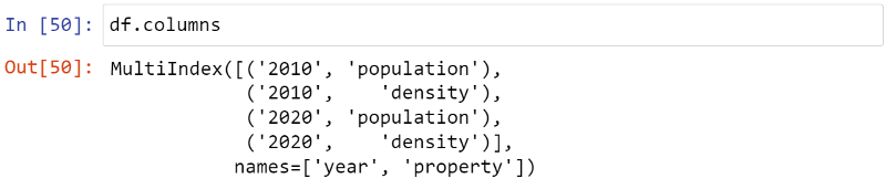
df.columns = df.columns.set_levels(df.columns.levels[0].astype(int), level=0)

But in order to use them properly, you need to understand what `levels` and `codes` are, and pdi allows you to use multi-indexing, just like you can use ordinary lists or NumPy arrays.

If you really want to know, `levels` and `codes` are what a regular list of tags of a particular level is broken down into to speed up operations like pivot, join, etc.:

pdi.get_level(df, 0) == Int64Index([2010, 2010, 2020, 2020])
df.columns.levels[0] == Int64Index([2010, 2020])
df.columns.codes[0] == Int64Index([0, 1, 0, 1])

Build a Dataframe with multiple indexes

Besides reading from CSV files and building from existing columns, there are ways to create multiple indexes. They are less commonly used - mostly for testing and debugging.

The most intuitive approach of using Panda's own multi-index representation doesn't work for historical reasons.

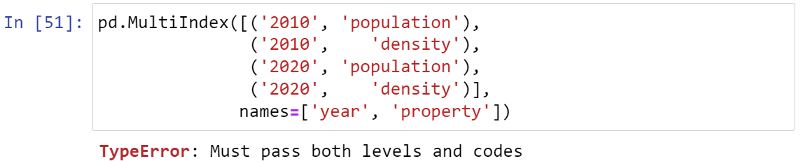
Here `Levels` and `codes` are (now) considered implementation details that should not be exposed to end users, but we have what we have.

Probably the easiest way to build a multiple index is as follows:

The disadvantage of this is that the name of the level must be specified on a separate line. There are several optional constructors that bundle names and labels together.

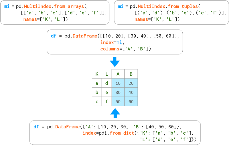
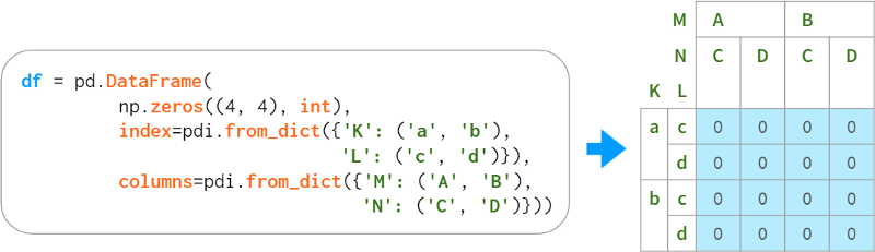
When levels form a regular structure, you can specify key elements and let Pandas automatically interweave them, like so:

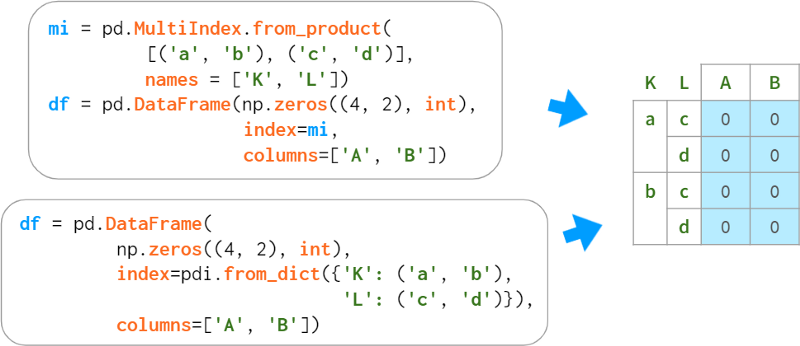
All methods listed above also apply to columns. For example:

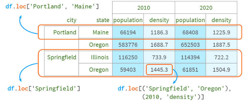
Indexing with multiple indexes

The benefit of accessing a DataFrame via a multiple index is that you can easily refer to all levels at once (possibly omitting inner levels) using familiar syntax.

Columns - via plain square brackets

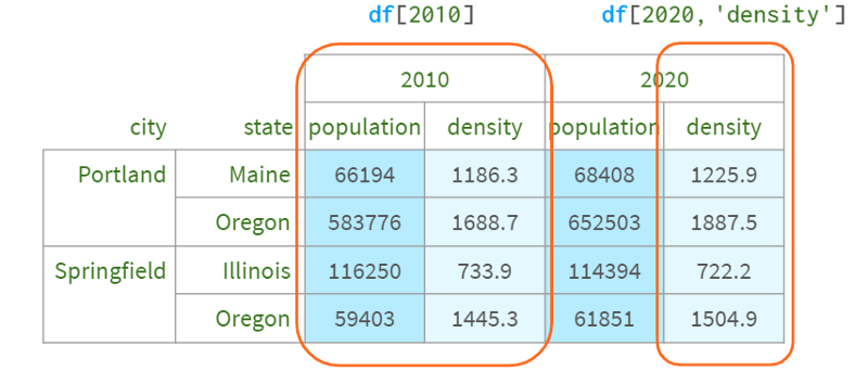
Rows and cells - use .loc[]

Now, what if you wanted to select all the cities in Oregon, or just leave the column with the population? The Python syntax has two limitations here.

1. There is no way to distinguish between df['a', 'b'] and df[('a', 'b')] - it is handled the same way, so you can't just write df[:,' Oregon ']. Otherwise, Pandas will never know whether you are referring to the column Oregon or the second level row Oregon

2. Python only allows colons in square brackets, not in parentheses, so you can't write df.loc[(:, 'Oregon'), :]

Technically, this is not difficult to arrange. I monkey-patched DataFrame to add such functionality, which you can see here:

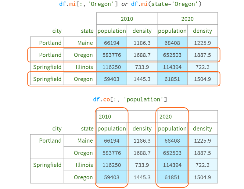
The only downside to this syntax is that it returns a copy when you use two indexers, so you can't write df.mi[:,'Oregon'] . Co['population'] = 10. There are many alternative indexers, some of which allow such assignments, but they all have their own characteristics:

1. You can swap inner with outer and use parentheses.

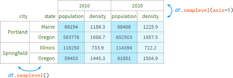
Thus, df[:, 'population'] can be implemented with df.swaplevel(axis=1)['population'] .

This feels hacky and inconvenient for more than two layers.

2. You can use the xs method: df.xs ('population', level=1, axis=1).

It doesn't feel very pythonic, especially when multiple levels are selected. This method cannot filter rows and columns at the same time, so the reason behind the name xs (which stands for "cross-section") is not entirely clear. It cannot be used to set a value.

3. You can create an alias for pd. idx = pd.IndexSlice; df.loc[:, idx[:, 'population']]

This is more pythonic, but to access elements, aliases have to be used, which is a bit cumbersome (the code without aliases is too long). You can select both rows and columns. writable.

4. You can learn how to use slice instead of colon. If you know that a[3:10:2] == a[slice(3,10,2)], then you may also understand the following code: df.loc[:, (slice(None), 'population' )], but it's barely readable. You can select both rows and columns. writable.

As a bottom line, Pandas has multiple ways of accessing elements of a DataFrame using multiple indexes using parentheses, but none of them are convenient enough, so they had to resort to another indexing syntax:

5. A mini-language for the .query method: df.query(' state=="Oregon" or city=="Portland" ').

It's convenient and fast, but lacks IDE support (no autocompletion, no syntax highlighting, etc.), and it only filters lines, not columns. This means that you can't implement df[:,'population'] with a DataFrame without transposing it (unless all columns are of the same type, which would result in loss of type). Non-writable.

Overlay and Split

Pandas does not have a set_index for columns. A common way to add hierarchies to a column is to "unstack" the existing hierarchies from the index:

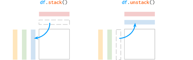
Pandas' stacks are very different from NumPy's stacks. Let's see what the documentation says about the naming convention:

"The function is named like a reorganized collection of books from horizontally positioned side by side (column of dataframe) to vertically stacked (in index of dataframe)."

The "on top" part doesn't sound convincing to me, but at least the explanation helps remember who moved things in which direction. By the way, Series has unstack, but not stack, because it's already "stacked". Since it is one-dimensional, Series can be used as a row vector or a column vector in different situations, but is generally considered a column vector (such as a dataframe column).

For example:

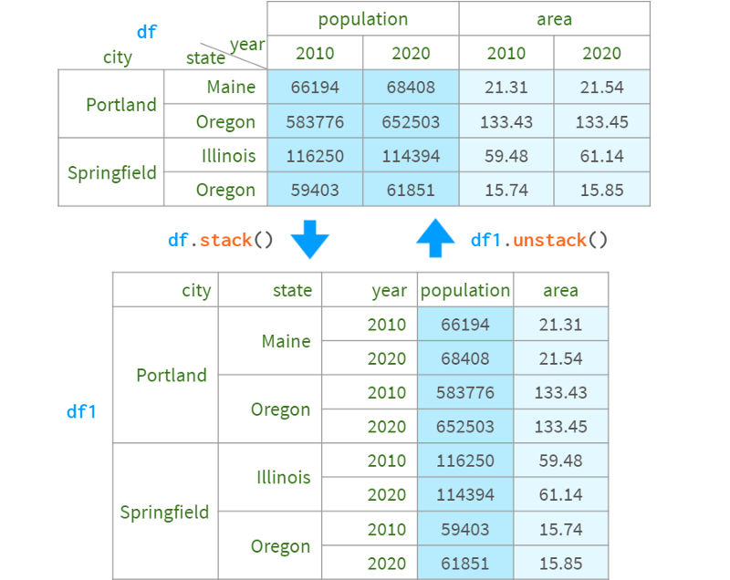
You can also specify the level to stack/unstack by name or position index. In this example, df.stack(), df.stack(1) and df.stack(' year ') produce the same the result of. The destination is always "after the last layer" and is not configurable. If you need to place the levels elsewhere, you can use df.swaplevel().sort_index() or pdi. swap_level (df = True)

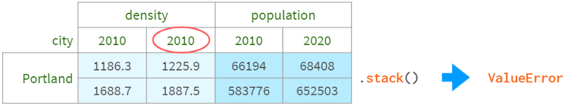
Columns must not contain duplicate values to be stackable (and so are indexes when unstacking):

How to prevent stacking/exploding sort

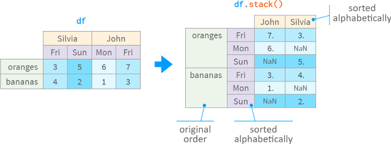
Both stack and unstack have a bad habit of unpredictably sorting the resulting index lexicographically. This can be irritating at times, but it's the only way to give predictable results when there are a lot of missing values.

Consider the following example. In what order do you want the days of the week to appear in the table on the right?

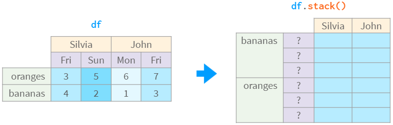
You can speculate that if John's Monday is to the left of John's Friday, then 'Mon' < 'Fri', similarly, Silvia's 'Fri' < 'Sun', so the result should be 'Mon' < 'Fri' < 'Sun'. This is legal, but what if the remaining columns are in a different order, like 'Mon' < 'frii' and 'Tue' < 'frii'? Or 'Mon' < 'friday' and 'Wed' < 'Sat' ?

Well, there aren't that many days in a week, and Pandas can infer the order based on prior knowledge. However, mankind has not yet come to a decisive conclusion whether Sunday should be the end or the beginning of the week. Which order should Pandas use by default? Read locales? What about less trivial orders, like the order of states in the US?

In this case, all Pandas does is simply sort alphabetically, as follows:

While this is a reasonable default, it still feels wrong. There should be a solution! There is one. It's called a CategoricalIndex. It remembers the order even if some tags are missing. It has recently been smoothly integrated into the Pandas toolchain. The only thing it lacks is infrastructure. It's hard to set up; it's brittle (falls back to objects in some operations), but it's perfectly usable, and the pdi library has some helpers that steepen the learning curve.

For example, to tell Pandas to lock the order of a simple index that stores products (which will inevitably happen if you decide to unstack the days of the week back into the column), you need to write horrible code like df . index = pd.CategoricalIndex(df.index) df index. index sort=True). It is more suitable for multi-index.

The pdi library has a helper function locked (and an alias lock which defaults to inplace=True ) to lock the ordering of a certain multi-index level by promoting it to a CategoricalIndex:

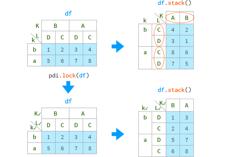
A check mark next to a level name indicates that the level is locked. It can be visualized manually using pdi.vis(df) or automatically visualized with monkey patches on the DataFrame HTML output using pdi.vis_patch(). After applying the patch, simply writing `df` in a Jupyter cell will show checkmarks for all levels of the lock order.

Lock and locked work automatically in simple cases (like client names), but require user prompts in more complex cases (like day of the week with missing dates).

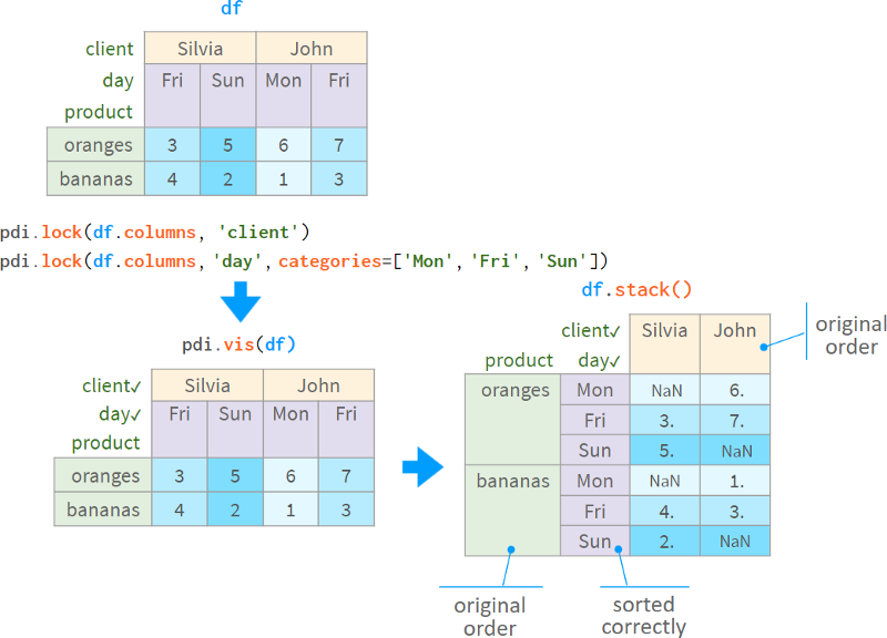
After the level is switched to CategoricalIndex, it will keep the original order in sort_index, stack, unstack, pivot, pivot_table and other operations.

However, it is fragile. Even something as simple as df['new_col'] = 1 will break it. Use pdi.insert(df.columns, 0, 'new_col', 1) to correctly handle levels with CategoricalIndex.

operating level

In addition to the previously mentioned methods, there are some other methods:

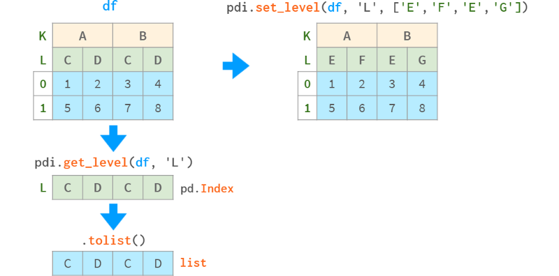
pdi.get_level(obj, level_id) returns a specific level referenced by number or name, available for DataFrames, Series and MultiIndex
pdi.set_level(obj, level_id, labels) replaces the labels of the level with the given array (list, NumPy array, Series, Index, etc.)

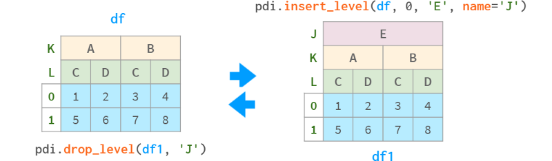
pdi.insert_level (obj, pos, labels, name) add a level with the given value (broadcast appropriately if necessary)
pdi.drop_level(obj, level_id) removes the specified level from the multi-index

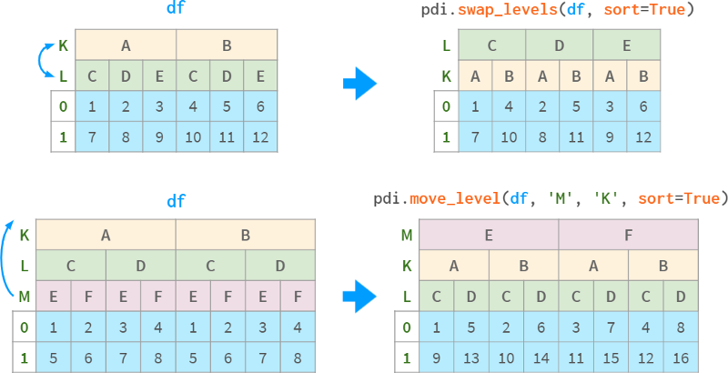
pdi.swap_levels (obj, src=-2, dst=-1) swap two levels (the default is the two innermost levels)

pdi.move_level (obj, src, dst) moves a specific level src to the specified position dst

In addition to the above parameters, all functions in this section have the following parameters:

axis=None where None means "column" for DataFrame and "index" for Series
sort=False, optional sort the corresponding multi-index after the operation
inplace=False, optionally perform the operation in-place (cannot be used for a single index as it is immutable).

All the operations above understand the word "level" in the traditional sense (the number of labels for a level is the same as the number of columns in the data frame), hiding the mechanism of indexing. labels and indexes. Code from end users.

In rare cases, when moving and swapping individual levels is not enough, you can use the pure Pandas call :df to reorder all the levels at once. columns = df.columns.reorder_levels([' M ', ' L ', ' K ']) where [' M ', ' L ', ' K '] is the desired order of the levels.

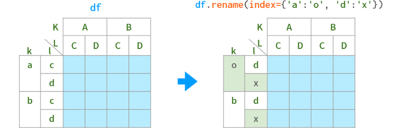
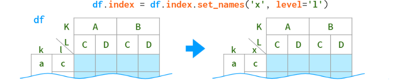
Usually it's enough to use get_level and set_level to fix the labels as necessary, but if you want to apply transformations to all levels of a multiindex at once, Pandas has a (ambiguously named) function rename that accepts a dict or a function:

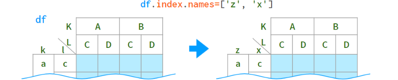
As for renaming levels, their names are stored in the .names field. The field does not support direct assignment (why not?): df.index.names[1] = ' x ' # TypeError, but can be replaced as a whole:

When you only need to rename a specific level, the syntax is as follows:

Convert a multi-index to a flat index and restore it

As we saw above, the convenience query method only addresses the complexity of dealing with multiple indexes on a row. Despite having so many helper functions, there can be a shocking effect for beginners when certain Pandas functions return multi-indexes on columns. So the pdi library has the following:

join_levels(obj, sep='_', name=None) join all multi-index levels to one index
split_level(obj, sep='_', names=None) splits the index back into multi-index

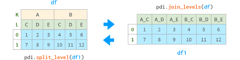
They both have optional axis and inplace parameters.

Sort MultiIndex

Since multi-indexes consist of multiple levels, sorting is more artificial than for single-indexes. This can still be done using the sort_index method, but can be further fine-tuned with the following parameters.

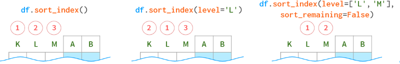
To sort on column level, specify axis=1.

Read and write multi-index dataframe to disk

Pandas can write a DataFrame with multiple indexes to a CSV file in a fully automated fashion: df.to_csv('df.csv') . But when reading such a file, Pandas cannot automatically resolve multiple indexes and needs some hints from the user. For example, to read a DataFrame with columns three levels high and an index four levels wide, you would specify pd.read_csv('df.csv', header=[0,1,2], index_col=[0,1,2, 3]).

This means that the first three rows contain information about the column, and the first four fields of each subsequent row contain the index level (if the column has more than one level, you can no longer refer to the row level by name, only by number).

Manually deciphering the number of layers in a multi-index is inconvenient, so a better idea is to stack() all column header layers before saving the DataFrame to CSV, and unstack() them after reading.

If you need a "forget it" solution, you might want to look into a binary format, such as Python's pickle format:

Direct call: df.to_pickle('df.pkl'), pd.read_pickle('df.pkl')

Use storemagic in Jupyter %store df then %store -r df (stored in $
HOME/.ipython/profile_default/db/autorestore)

Python's pickle is small and fast, but only accessible within Python. If you need to interoperate with other ecosystems, look at more standard formats like the Excel format (requires the same hint as read_csv when reading MultiIndex). code show as below:

!pip install openpyxl  
df.to_excel('df3.xlsx')  
df.to_pd.read_excel('df3.xlsx', header=[0,1,2], index_col=[0,1,2,3])

Or look at other options (see docs).

MultiIndex Arithmetic

When using a multi-index data frame, the same rules apply as for normal data frames (see above). But processing a subset of cells has some properties of its own.

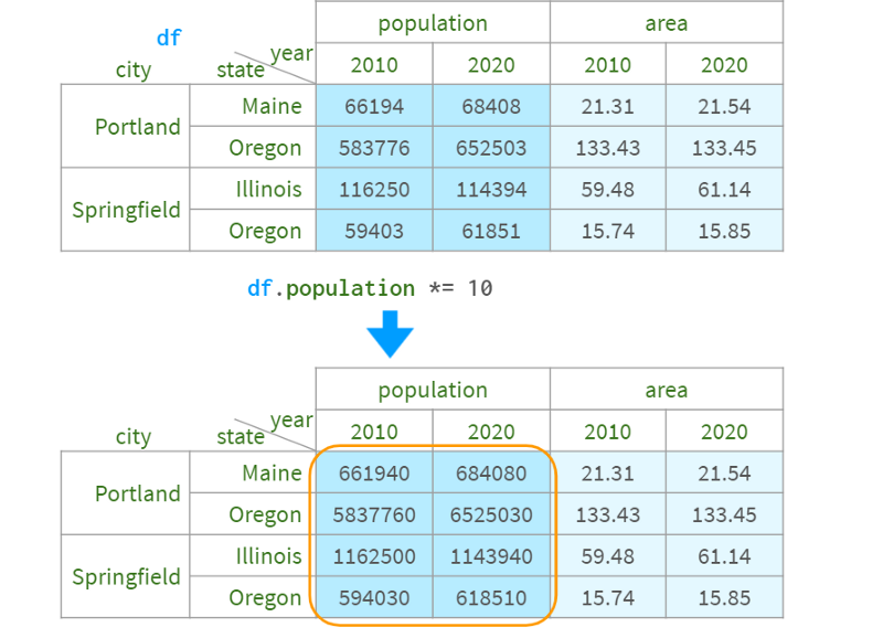
Users can update some columns through the external multi-index level, as follows:

If you want to keep the original data unchanged, you can use df1 = df.assign(population=df.population*10).

You can also easily get the population density with density=df.population/df.area.

But unfortunately, you cannot assign the result to the original dataframe with df.assign.

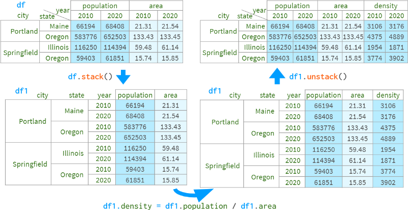
One approach is to stack all unrelated levels of the column index into the row index, perform the necessary calculations, and then unstack them back (using pdi). lock to preserve the original order of the columns).

Alternatively, you can also use pdi.assign:

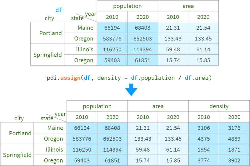
pdi.assign is lock order aware, so if you give it a dataframe with one (multiple) lock levels, it won't unlock them or the subsequent stack/unstack/etc. Operations will maintain the original column and row order.

All in all, Pandas is a great tool for analyzing and manipulating data. Hope this article helps you understand the "how" and "why" of solving typical problems, and appreciate the true value and beauty of the Pandas library.

Finally, recommend your own column

Learning GPT alone is time-consuming and laborious, and there is no one to discuss, communicate and guide when encountering problems, wasting a lot of time and energy. Now the top priority is to use this super AI quickly and quickly to help you improve the efficiency of work and study and save costs!

The original price is 299, and the current early bird price is 109 yuan (the content is permanently valid), and the price will be adjusted tonight! If it is over 200, it will increase by 20, and it will continue to rise to the original price . At present, many planets are priced at hundreds of dollars. WeChat contact editor: coder_v5

At present, there are still a small number of GPT accounts with 5 dollars in them (the password can be changed), and everyone knows that registration is getting more and more difficult. The market price of this account has been fired up to 40 yuan a piece. We will send this independent account to students who sign up for our column!