Table of contents

1.1 Evolution of Wireless Communication Technology

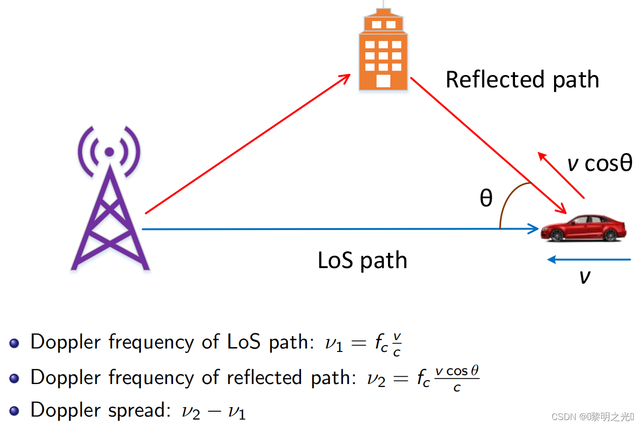
1.3 Wireless channel - Doppler spread

1.4 Typical time delay and Doppler shift

1.5 Conventional modulation scheme - OFDM

2. OTFS

2.1 Problems of OFDM

2.2 Introduction to OTFS

Received signal in a linear time-varying channel (LTV)

The relationship between h(τ,ν) and H(t,f)

2.3 OTFS Modulation

3. OTFS architecture compatible with OFDM

Appendix: Notes on my push formula

1. Introduction

1.1 Evolution of Wireless Communication Technology

Waveform design is a major change between each generation of digital communication systems

1.2 Wireless channel - delay extension

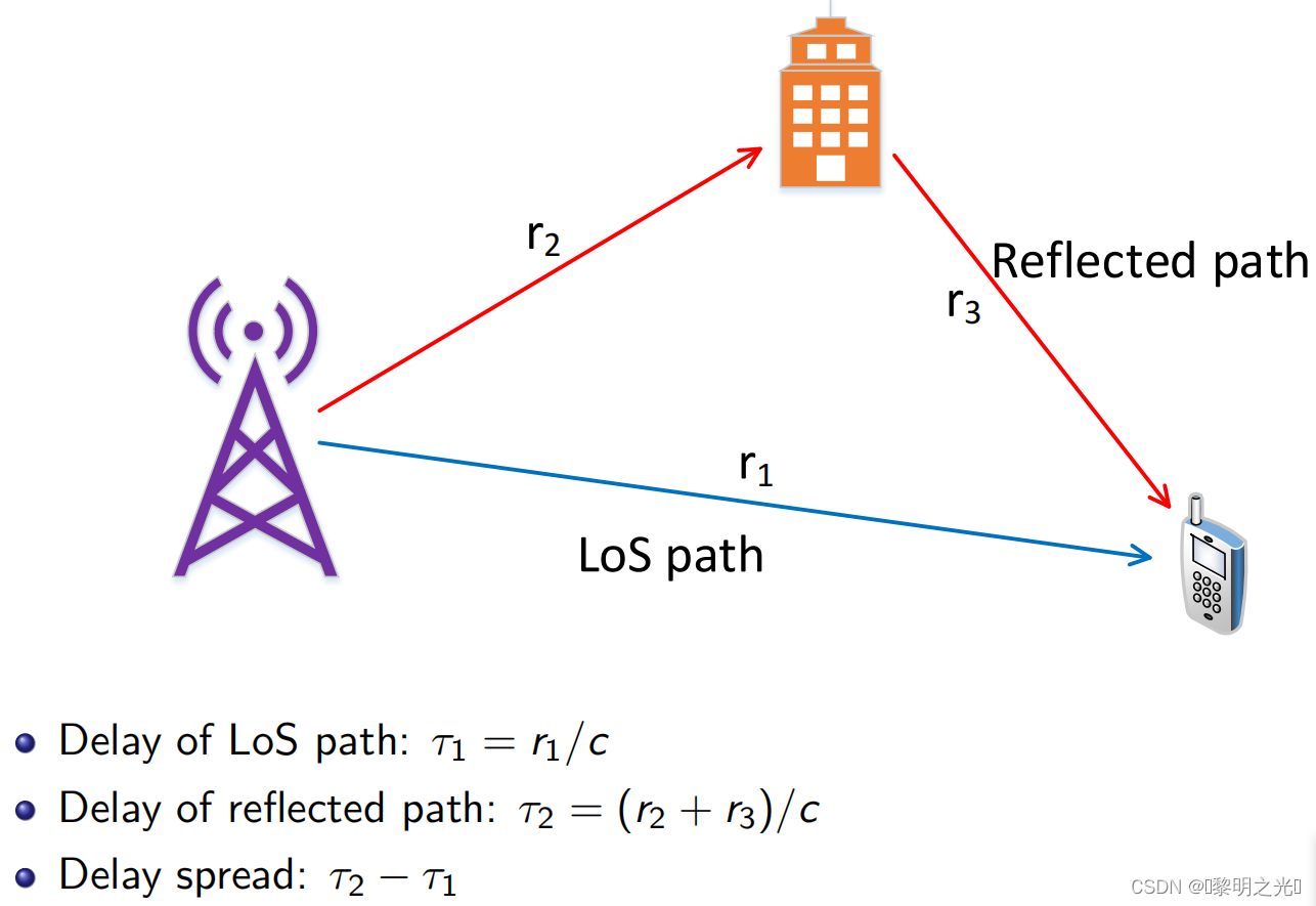
The bandwidth of the channel is related to the relative delay of the two paths, which is called the delay spread of the multipath . Extending the above model to the scenario where there are multiple paths between the transceivers, the corresponding channel bandwidth can be roughly expressed as

When the signal bandwidth is greater than the channel bandwidth

After the signal propagates through the wireless channel, some frequency signals can pass through, while some frequency signals are severely attenuated, causing the overall signal to be distorted. To overcome this problem, 2G systems use narrowband signals (the bandwidth of the signal is 200KHz). However, due to the small bandwidth of the narrowband signal, the data rate it can carry is limited. Both 3G and 4G cellular networks are broadband communication systems to provide high transmission data rates. Obviously, broadband communication systems need to overcome the situation that "signal bandwidth is greater than channel bandwidth". Both CDMA and OFDM can overcome the above phenomenon, but because CDMA technology was independently developed by Qualcomm, which owns no less than 75% of the CDMA core patents, continuing to use CDMA technology in the 3G system in the 4G system will cause wireless operators to rely on Qualcomm. Pay high patent fees. However, OFDM was designed by Bell Laboratories in 1966, and its patent protection has long since expired, so it has received strong support from wireless equipment manufacturers and operators. Finally, in the process of 4G network standardization, 3GPP-led LTE with OFDM as the core defeated UWB (Ultra Wide Band, ultra-wideband technology) with CDMA as the core led by 3GPP2 (Qualcomm) and became the core of the 4G broadband communication access network. technology.

1.3 Wireless channel - Doppler spread

Among them, the Doppler frequency shift fd is the Doppler frequency, which is proved as follows

But note: this is different from the Doppler frequency calculated by the radar, because the radar is a round-trip process, and the final result needs to be multiplied by 2 (twice the one-way path).

1.4 Typical time delay and Doppler shift

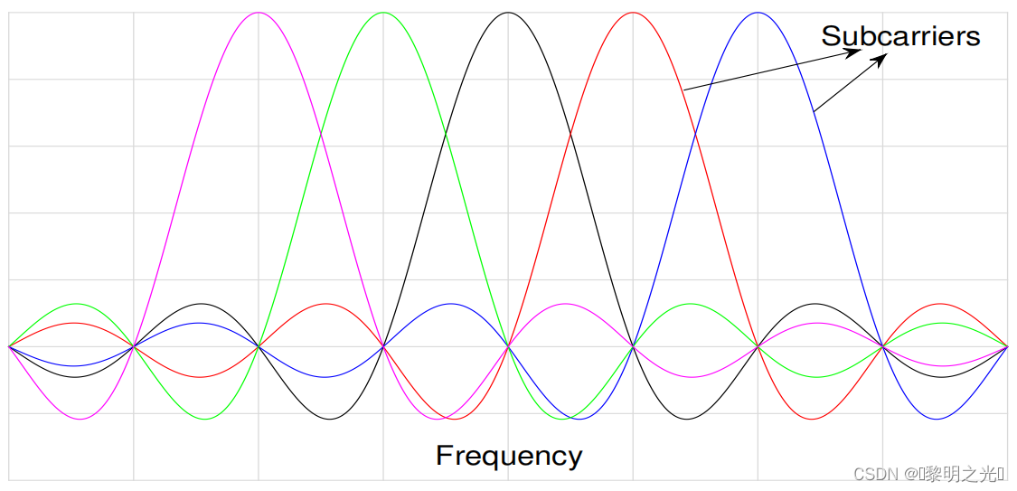
1.5 Conventional modulation scheme - OFDM

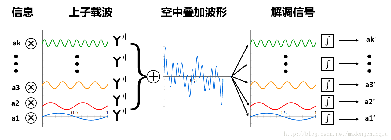
The core idea of OFDM technology is to divide a wide frequency carrier into multiple orthogonal subcarriers with smaller bandwidths , as shown in the figure below, and use these orthogonal subcarriers to send and receive signals. Since the bandwidth of each subcarrier is smaller than the channel bandwidth, OFDM can effectively overcome frequency selective fading. Since multiple carriers are used for signal transmission at the same time, OFDM technology is a kind of multi-carrier transmission technology. Next, I will use a mathematical model to explain the principle of OFDM transmission signals.

First of all, you need to understand the principle of OFDM, refer to the following article:

The relationship between OFDM and FFT

Consider an N subcarrier OFDM system

The parameters are defined as follows:

$N$ : Indicates the number of subcarriers

$\Delta f=1/T$ : Indicates the subcarrier spacing

$B=N\Delta f$ : total bandwidth of OFDM signal

$T_{cp}$ : the duration of the cyclic prefix

$T_{s}$ : sampling interval, $T_{s}=1/f_{s}=1/B$

$f_{s}$ : Sampling frequency

$T_{u}$ : effective data symbol time (OFDM symbol), $T_{u}=NT_{s}$

$T=T_{u}+T_{cp}$ OFDM symbol length

If the center frequency of the first carrier is $f_{0}$ , the frequency of n carriers is $f_{n}=f_{0}+(n-1)\Delta f$ .

An OFDM-based multi-carrier modulated transmission signal is defined by the following formula (multi-carrier superposition)

[Formula 1]

Xn is a row vector, which can be expressed as $[X_{1},..,X_{n},...,X_{N}]$ , each column vector $X_{i}$ represents the transmission symbol on the i-th carrier.

Assuming that the subcarrier interval Δf=15kHz, the transmission time of an OFDM symbol is 66.7us, it can be found that 15kHz*66.67us=1, that is, the transmission time of an OFDM symbol on the baseband is just to send a complete waveform of the first harmonic. For the 10M LTE system, 1024 subcarriers are used, but only the middle 600 subcarriers (excluding the middle DC) are used to transmit data. Within the time of one OFDM symbol (ie 66.67us), the two first harmonics close to the middle transmit a complete waveform, and the two second harmonics at the outer point transmit two complete waveforms, and so on to the outermost The two 300th harmonics transmit 300 complete waveforms. Within the 66.67us, 600 subcarriers are orthogonal to each other, and 600 complex signals are respectively carried on them.

Speaking of this, looking at OFDM from the time domain, it is actually quite concise and pleasing. However, it is too difficult for a system to implement OFDM in the time domain. Time delay and frequency offset will seriously damage the orthogonality of subcarriers, thereby affecting system performance. At the same time, each carrier needs a crystal oscillator to generate the corresponding frequency. When the number of carriers is large enough (for example, 4G LTE has 1024 carriers), the cost of generating baseband signals will be high. Therefore, the realization of an OFDM system needs to start from the frequency domain .

By sampling the above formula, a discrete representation can be obtained, where the sampling interval is T (T=1/B), and the discrete representation of the lth sampling point is as follows:

[Official 2]

The maximum value of l is N, and for a given value of l, the right formula will uniquely determine a value. Therefore, all the results of l from 1 to N can be calculated, that is, $[\hat{f(1)},\hat{f(2)},...,\hat{f(lT)},...,\hat{f(N)}]$ they are all uniquely determined.

$[\hat{f(1)},\hat{f(2)},...,\hat{f(lT)},...,\hat{f(N)}]$ The value of the lth data point in [Formula 2] can be understood as $[X_{1},..,X_{n},...,X_{N}]$ the inverse discrete Fourier transform IFFT of [Formula 1]. Refer to the discrete Fourier transform formula:

Similarly, after receiving the N discrete data points at the receiving end $[\hat{f(1)},\hat{f(2)},...,\hat{f(lT)},...,\hat{f(N)}]$ , the original data symbols can be obtained after discrete Fourier transform (FFT) is performed on them $[X_{1},..,X_{n},...,X_{N}]$ . But have you noticed a problem: discrete Fourier transform and inverse discrete Fourier transform are DFT and IDFT that do not match the above FFT/IFFT. reason:

Because $[X_{1},..,X_{n},...,X_{N}]$ it is a discrete data point (discrete in time domain), it corresponds to the discrete Fourier transform DFT, but because FFT is actually a fast Fourier transform of DFT that simplifies the computational complexity , it is based on the discrete Fourier transform. Odd, Even, imaginary, real and other characteristics, obtained by improving the algorithm of discrete Fourier transform. In the software field, the complexity can be reduced to O(N*N) of DFT to O(nlogn) (if it is a two-dimensional image, it should be O( M*N*log(M*N) ), so we use FFT Replace it with IFFT to reduce complexity and improve computing performance.

Therefore, when the OFDM transceiver can be expressed as the following figure

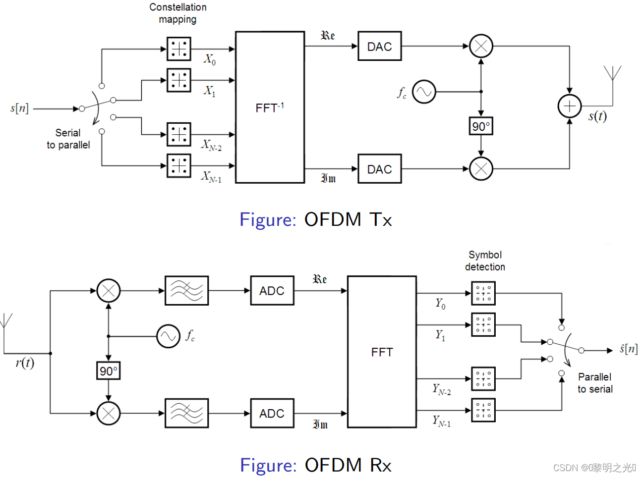
In implementing OFDM by IFFT, an IFFT module is added at the transmitting end, and an FFT module is added at the receiving end. The function of the IFFT module is equivalent to saying: Don’t bother sending N subcarrier signals, I can directly calculate what you will superimpose in the air in a discrete state, which is also convenient for me to use digital signals for signal processing; the function of the FFT module is quite Yu said: Don't use the old-fashioned integration method to remove the remaining orthogonal subcarriers, let me help you calculate all the N discrete data points carrying signals at a time. That's it, IFFT realizes the OFDM system using "mathematical method" to calculate the superimposed waveform of the signal at the sending end, and remove the orthogonal subcarrier at the receiving end, thus greatly simplifying the complexity of the system.

my notes:

For more, please refer to:

OFDM (Orthogonal Frequency Division Multiplexing) Technology - Zhihu (zhihu.com) https://zhuanlan.zhihu.com/p/137712898 OFDM complete simulation process and explanation (MATLAB) - Zhihu (zhihu.com) https: //zhuanlan.zhihu.com/p/57967971

2. OTFS

2.1 Problems of OFDM

Inter-subcarrier interference (ICI)
Subchannel gains are not equal, lowest gain determines performance
Multiple Dopplers are hard to balance
When the channel is not ideal or in a high Doppler environment, the channel matrix matrix loses its cyclic structure and the decomposition becomes an error

2.2 Introduction to OTFS

Solve the problem of OFDM
Works in the delay-Doppler domain, not the time-frequency domain

Different channel representations in linear time-varying channels: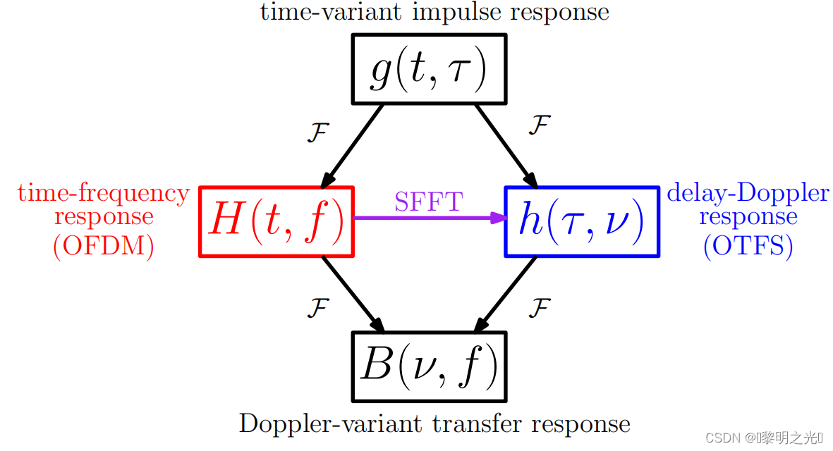

Received signal in a linear time-varying channel (LTV)

time-varying channel impulse response

Delay-Doppler domain channel function

Time-Frequency Domain Channel Response

The relationship between h(τ,ν) and H(t,f)

The image is represented as:

Therefore, the relationship between the DD domain and the TF domain can be related by SFFT and ISFFT, that is, OTFS and OFDM are inextricably linked

Based on the diagram above, I will provide below some knowledge about the three domains involved: discrete time domain, time-frequency domain and delay-Doppler domain:

We assume that the OTFS system operates on a high-mobility channel containing p paths, with a bandwidth of B, a maximum delay spread τmax and a maximum Doppler shift νmax. We consider a discrete-time baseband equivalent model in which a continuous-time OTFS signal $f_{s}=B=1/T_{s}$ is sampled at a sampling frequency where $T_{s}$ denoted sampling interval is the duration of each OTFS symbol. The discrete time-domain OTFS frame includes N*M sampling points, M represents the number of subcarriers, and N represents the number of OTFS symbols in each block. Thus, the OTFS frame duration is $T_{f}=NMT_{s}=MT$ , where $T=NT_{s}$ denotes the duration of each block.

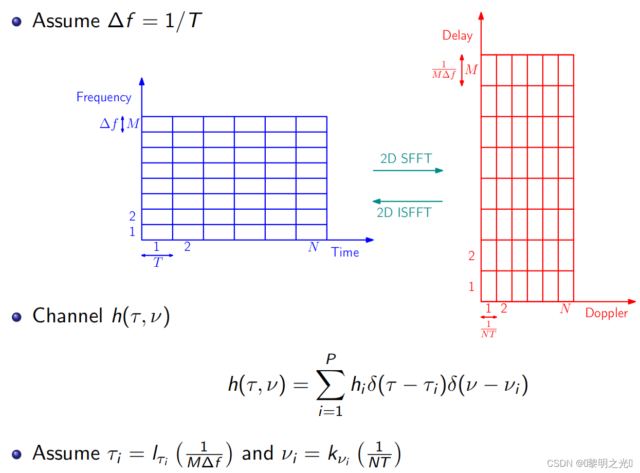
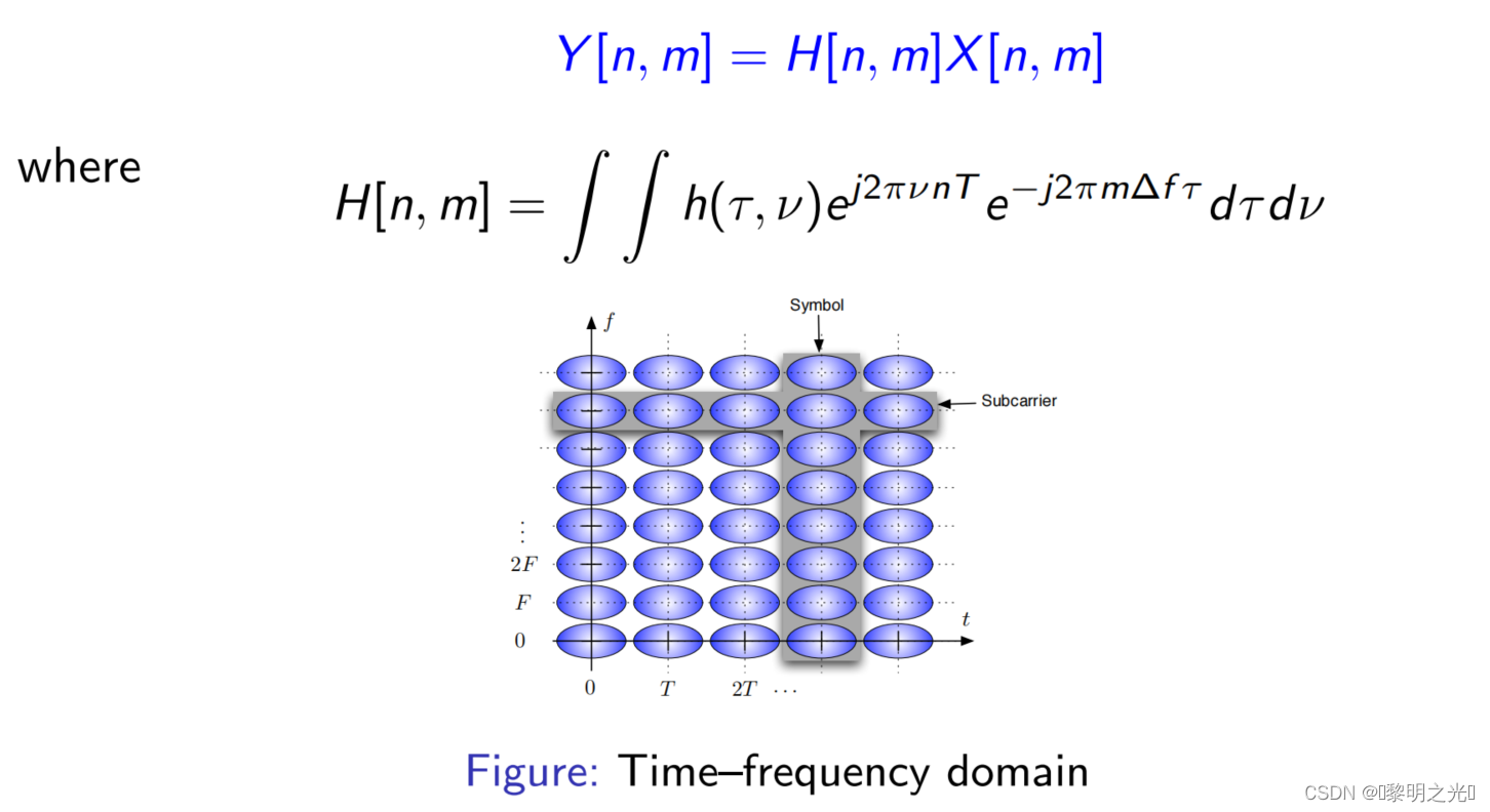
Every $T$ second, we perform M-point discrete Fourier transform (DFT) on each block to obtain the discrete spectrum of each block, where the spectral interval is $\Delta f=1/T$ . $B=M\Delta f$ All spectra of the bandwidth of the OTFS frame are collected along the time axis $N$ , defining the discrete time-frequency domain, as shown in the figure above (left). The discrete time-frequency domain is defined as an array of M×N points which can be expressed as $X_{tf}[l,k],l=0,1,2,...,M-1,k=0,1,2,...,N-1$ . Each column contains discrete spectral samples for each block. We can conveniently regard this matrix as the two-dimensional time-frequency representation of the one-dimensional time-domain OTFS signal, and the two-dimensional time-frequency domain grid $\Lambda$ can be expressed as:

$\Lambda =[(l\Delta f,kT),l=0,...,M-1,k=0,...,N-1]$

Discrete time-frequency domain samples can be transformed into time-delay-Doppler domain by two-dimensional symplectic Fourier transform. Specifically, the time-delay-Doppler domain is obtained by inverse Fourier transform along the frequency axis ( $X_{tf}[l,k]$ performed on columns) and along the time axis ( performed on rows). $X_{tf}[l,k]$ The corresponding M×N point array in the discrete delay-Doppler domain is shown on the right side of the figure above, and the two-dimensional delay-Doppler domain grid $\Gamma$ can be defined as the following formula

$\Gamma =[(\frac{m}{M\Delta f},\frac{n}{NT}),m=0,...,M-1,n=0,...,N-1]$

where $\frac{1}{M\Delta f}$ and are $\frac{1}{NT}$ the resolutions of path delay and Doppler shift. In particular, $\frac{1}{M\Delta f}$ two paths with the same Doppler shift but less difference in propagation delay cannot be distinguished by the receiver. Likewise, two paths with the same propagation delay but less difference in Doppler shift $\frac{1}{NT}$ are indistinguishable. The notation of the simultaneous delay-Doppler domain can be expressed as $X[m,n],m=0,...,M-1,n=0,...,N-1$

Typical OTFS parameters are as follows:

2.3 OTFS Modulation

The time-frequency domain in the figure is similar to an OFDM system with N symbols in the data frame (pulse-shaped OFDM)

OTFS modulation principle:

OTFS modulation

At the OTFS transmitter side, the information symbols are first mapped to the DD domain. The inverse symplectic finite Fourier transform (ISFFT) is used to transform the DD domain symbol x[k,l] into the TF domain symbol X[n,m].

[Official 2.3.1]

Then, through the Heisenberg transformation of X[n,m], the time domain signal s (t) can be obtained.

[Official 2.3.2]

gtx (t) indicates the transmitted pulse waveform

Tips：

The ISFFT above can be viewed as an n-point fft along each Doppler axis and an m-point ifft along each delay axis

channel

[Official 2.3.3]

OTFS Demodulation (Matched Filter) - Wigner Transform

At the OTFS receiving end, first use the Wigner transform to convert the received time domain signal r (t) into a TF domain symbol Y [n, m], this process is also called Match filter (Match filter)

[Official 2.3.4]

[Official 2.3.5/2.3.6]

grx (t) represents the received pulse waveform, if gtx (t) and grx (t) are rectangular pulses, then [2.3.2] and [2.3.4] are simplified as a set of M-point IFFT and FFT respectively, and further , when N = 1, the above two formulas are equivalent to OFDM modulation and demodulation respectively.

If the transmitted and received pulses gtx (t) and grx (t) are ideal pulses that satisfy the biorthogonal property (the time domain and the frequency domain do not overlap), symbol interference can be eliminated. In the case of biorthogonality, the input of the time-frequency domain The output relation can be expressed as:

H[n,m] can be discretized as

The DD domain is then symbol-demodulated using the symplectic finite Fourier transform (SFFT).

Symplectic finite Fourier transform

[Official 2.3.7]

The ISFFT above can be viewed as an m-point ifft along each Doppler axis and an n-point fft along each delay axis

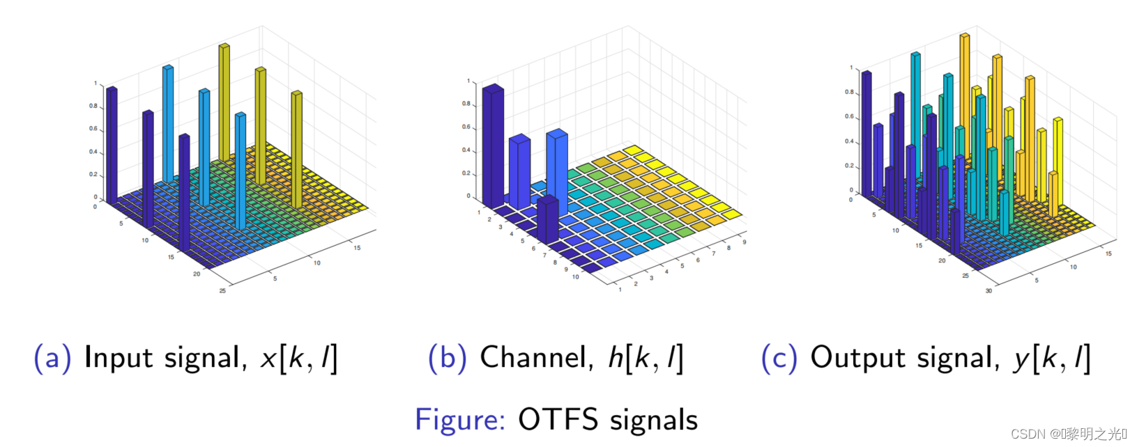
On the DD domain, formula [2.3.7] can be further expressed as:

Among them, the two-dimensional image of the input and output and the channel is as follows

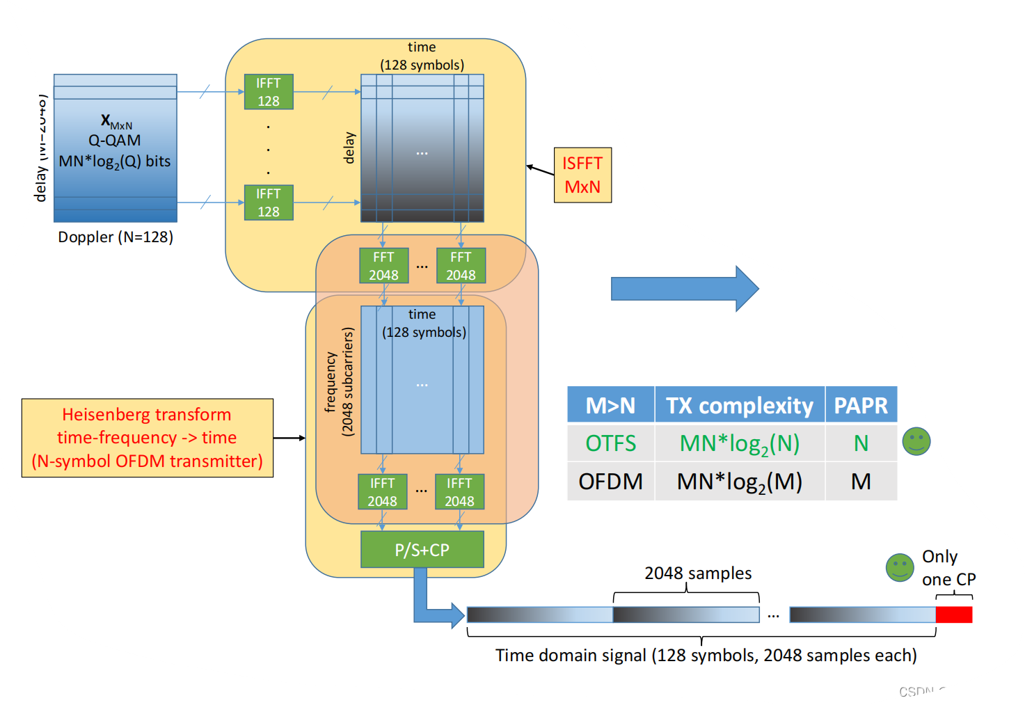
3. OTFS architecture compatible with OFDM

When the input and output waveforms gtx and grx are rectangular pulses and N=1, Heisenberg transform and Wigner transform are equivalent to OFDM modulation (IFFT) and demodulation (FFT)
OTFS compatible with LTE system
OTFS can be easily implemented by applying a precoding and decoding block to N consecutive OFDM symbols

But when the input and output waveforms gtx and grx are rectangular pulses, it is no longer a bi-orthogonal situation in the time-frequency domain, which means that there will be interference in both the time domain and the frequency domain

Time domain: ISI - loss of time domain orthogonality due to delay

Frequency Domain: ICI - Loss of Orthogonality in Frequency Domain due to Doppler

Therefore, in the case of OFDM, the input-output relationship can be modified as:

Appendix: Notes on my push formula

Similarities and differences between OTFS and OFDM

1. Introduction

1.1 Evolution of Wireless Communication Technology

1.2 Wireless channel - delay extension

1.3 Wireless channel - Doppler spread

1.4 Typical time delay and Doppler shift

1.5 Conventional modulation scheme - OFDM

2. OTFS

2.1 Problems of OFDM

2.2 Introduction to OTFS

Received signal in a linear time-varying channel (LTV)

The relationship between h(τ,ν) and H(t,f)

2.3 OTFS Modulation

3. OTFS architecture compatible with OFDM

Appendix: Notes on my push formula

Guess you like